Detailed Explanation of Digital Currency Pair Trading Strategy

Introduction

Recently, I saw BuOu’s Quantitative Diary mentioning that you can use negatively correlated currencies to select currencies, and open positions to make profits based on price difference breakthroughs. Digital currencies are basically positively correlated, and only a few currencies are negatively correlated, often with special market conditions, such as the independent market conditions of MEME coins, which are completely different from the market trend. These currencies can be selected and go long after the breakthrough. This method can make profits under specific market conditions. However, the most common method in the field of quantitative trading is to use positive correlation for paired trading. This article will introduce this strategy briefly.

Digital currency pair trading is a trading strategy based on statistical arbitrage, which simultaneously buys and sells two highly correlated cryptocurrencies to obtain profits from price deviations. This article will introduce the principles of this strategy, profit mechanism, methods of selecting currencies, potential risks and ways to improve them, and provide some practical Python code examples.

Strategy Principle

Pair trading strategies rely on the historical correlation between the prices of two digital currencies. When the prices of two currencies show a strong correlation, their price trends are generally in sync. If the price ratio between the two deviates significantly at a certain moment, it can be considered a temporary abnormality and the price will tend to return to normal levels. The digital currency market is highly interconnected. When a major digital currency (such as Bitcoin) fluctuates significantly, it will usually trigger a coordinated reaction in other digital currencies. Some currencies may have a very obvious positive correlation that can last due to the same investment institutions, the same market makers, and the same track. Some currencies are negatively correlated, but there are fewer negatively correlated currencies, and since they are all affected by the market trend, they will often have consistent market trends.

Assume that currency A and currency B have a high price correlation. At a certain moment, the average value of the A/B price ratio is 1. If at a certain moment, the A/B price ratio deviates by more than 0.001, that is, more than 1.001, then you can trade in the following ways: Open a long position on B and open a short position on A. On the contrary, when the A/B price ratio is lower than 0.999: Open a long position on A and open a short position on B.

The key to profitability lies in the spread gains when prices deviate from the mean and return to normal. Since price deviations are usually short-lived, traders can close their positions when prices return to the mean and profit from the spread.

Prepare the Data

Import the corresponding library

These codes can be used directly. It is best to download Anancoda and debug it in Jupyer notebook. It includes packages for commonly used data analysis directly.

import requests
from datetime import date,datetime
import time
import pandas as pd
import numpy as np
import matplotlib.pyplot as plt
import requests, zipfile, io
%matplotlib inline

Get all trading pairs being traded

Info = requests.get('https://fapi.binance.com/fapi/v1/exchangeInfo')
b_symbols = [s['symbol'] for s in Info.json()['symbols'] if s['contractType'] == 'PERPETUAL' and s['status'] == 'TRADING' and s['quoteAsset'] == 'USDT']
b_symbols = list(filter(lambda x: x[-4:] == 'USDT', [s.split('_')[0] for s in b_symbols]))
b_symbols = [x[:-4] for x in b_symbols]
print(b_symbols) # Get all trading pairs being traded

Download K-line function

The main function of the GetKlines function is to obtain the historical K-line data of the specified trading pair perpetual contract from the Binance exchange and store the data in a Pandas DataFrame. The K-line data includes information such as opening price, highest price, lowest price, closing price, and trading volume. This time we mainly use the closing price data.

def GetKlines(symbol='BTCUSDT',start='2020-8-10',end='2024-7-01',period='1h',base='fapi',v = 'v1'):
    Klines = []
    start_time = int(time.mktime(datetime.strptime(start, "%Y-%m-%d").timetuple()))*1000 + 8*60*60*1000
    end_time =  min(int(time.mktime(datetime.strptime(end, "%Y-%m-%d").timetuple()))*1000 + 8*60*60*1000,time.time()*1000)
    intervel_map = {'m':60*1000,'h':60*60*1000,'d':24*60*60*1000}
    while start_time < end_time:
        time.sleep(0.3)
        mid_time = start_time+1000*int(period[:-1])*intervel_map[period[-1]]
        url = 'https://'+base+'.binance.com/'+base+'/'+v+'/klines?symbol=%s&interval=%s&startTime=%s&endTime=%s&limit=1000'%(symbol,period,start_time,mid_time)
        res = requests.get(url)
        res_list = res.json()
        if type(res_list) == list and len(res_list) > 0:
            start_time = res_list[-1][0]+int(period[:-1])*intervel_map[period[-1]]
            Klines += res_list
        if type(res_list) == list and len(res_list) == 0:
            start_time = start_time+1000*int(period[:-1])*intervel_map[period[-1]]
        if mid_time >= end_time:
            break
    df = pd.DataFrame(Klines,columns=['time','open','high','low','close','amount','end_time','volume','count','buy_amount','buy_volume','null']).astype('float')
    df.index = pd.to_datetime(df.time,unit='ms')
    return df

Download data

The data volume is relatively large. In order to download faster, only the hourly K-line data of the last three months is obtained. df_close contains the closing price data of all currencies.

start_date = '2024-04-01'
end_date   = '2024-07-05'
period = '1h'
df_dict = {}

for symbol in b_symbols:   
    print(symbol)
    if symbol in df_dict.keys():
        continue
    df_s = GetKlines(symbol=symbol+'USDT',start=start_date,end=end_date,period=period)
    if not df_s.empty:
        df_dict[symbol] = df_s
df_close = pd.DataFrame(index=pd.date_range(start=start_date, end=end_date, freq=period),columns=df_dict.keys())
for symbol in symbols:
    df_close[symbol] = df_dict[symbol].close
df_close = df_close.dropna(how='all')

Backtesting Engine

We define an exchange object for the following backtest.

class Exchange:
    def __init__(self, trade_symbols, fee=0.0002, initial_balance=10000):
        self.initial_balance = initial_balance #Initial assets
        self.fee = fee
        self.trade_symbols = trade_symbols
        self.account = {'USDT':{'realised_profit':0, 'unrealised_profit':0, 'total':initial_balance,
                                'fee':0, 'leverage':0, 'hold':0, 'long':0, 'short':0}}
        for symbol in trade_symbols:
            self.account[symbol] = {'amount':0, 'hold_price':0, 'value':0, 'price':0, 'realised_profit':0,'unrealised_profit':0,'fee':0}
            
    def Trade(self, symbol, direction, price, amount):
        cover_amount = 0 if direction*self.account[symbol]['amount'] >=0 else min(abs(self.account[symbol]['amount']), amount)
        open_amount = amount - cover_amount
        self.account['USDT']['realised_profit'] -= price*amount*self.fee #Deduction fee
        self.account['USDT']['fee'] += price*amount*self.fee
        self.account[symbol]['fee'] += price*amount*self.fee
        if cover_amount > 0: #Close the position first
            self.account['USDT']['realised_profit'] += -direction*(price - self.account[symbol]['hold_price'])*cover_amount  #profit
            self.account[symbol]['realised_profit'] += -direction*(price - self.account[symbol]['hold_price'])*cover_amount
            self.account[symbol]['amount'] -= -direction*cover_amount
            self.account[symbol]['hold_price'] = 0 if self.account[symbol]['amount'] == 0 else self.account[symbol]['hold_price']
        if open_amount > 0:
            total_cost = self.account[symbol]['hold_price']*direction*self.account[symbol]['amount'] + price*open_amount
            total_amount = direction*self.account[symbol]['amount']+open_amount
            
            self.account[symbol]['hold_price'] = total_cost/total_amount
            self.account[symbol]['amount'] += direction*open_amount      
    
    def Buy(self, symbol, price, amount):
        self.Trade(symbol, 1, price, amount)
        
    def Sell(self, symbol, price, amount):
        self.Trade(symbol, -1, price, amount)
        
    def Update(self, close_price): #Update the assets
        self.account['USDT']['unrealised_profit'] = 0
        self.account['USDT']['hold'] = 0
        self.account['USDT']['long'] = 0
        self.account['USDT']['short'] = 0
        for symbol in self.trade_symbols:
            if not np.isnan(close_price[symbol]):
                self.account[symbol]['unrealised_profit'] = (close_price[symbol] - self.account[symbol]['hold_price'])*self.account[symbol]['amount']
                self.account[symbol]['price'] = close_price[symbol]
                self.account[symbol]['value'] = self.account[symbol]['amount']*close_price[symbol]
                if self.account[symbol]['amount'] > 0:
                    self.account['USDT']['long'] += self.account[symbol]['value']
                if self.account[symbol]['amount'] < 0:
                    self.account['USDT']['short'] += self.account[symbol]['value']
                self.account['USDT']['hold'] += abs(self.account[symbol]['value'])
                self.account['USDT']['unrealised_profit'] += self.account[symbol]['unrealised_profit']
        self.account['USDT']['total'] = round(self.account['USDT']['realised_profit'] + self.initial_balance + self.account['USDT']['unrealised_profit'],6)
        self.account['USDT']['leverage'] = round(self.account['USDT']['hold']/self.account['USDT']['total'],3)

Correlation Analysis to Filter Currencies

Correlation calculation is a method in statistics used to measure the linear relationship between two variables. The most commonly used correlation calculation method is the Pearson correlation coefficient. The following is the principle, formula and implementation method of correlation calculation. The Pearson correlation coefficient is used to measure the linear relationship between two variables, and its value range is between -1 and 1:

• 1 indicates a perfect positive correlation, where the two variables always change in sync. When one variable increases, the other also increases proportionally. The closer it is to 1, the stronger the correlation.
• -1 indicates a perfect negative correlation, where the two variables always change in opposite directions. The closer it is to -1, the stronger the negative correlation.
• 0 means no linear correlation, there is no straight line relationship between the two variables.

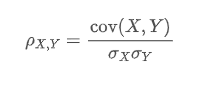
The Pearson correlation coefficient determines the correlation between two variables by calculating their covariance and standard deviation. The formula is as follows:

in which:

• is the Pearson correlation coefficient between variables X and Y.
• is the covariance of X and Y.
• and are the standard deviations of X and Y respectively.

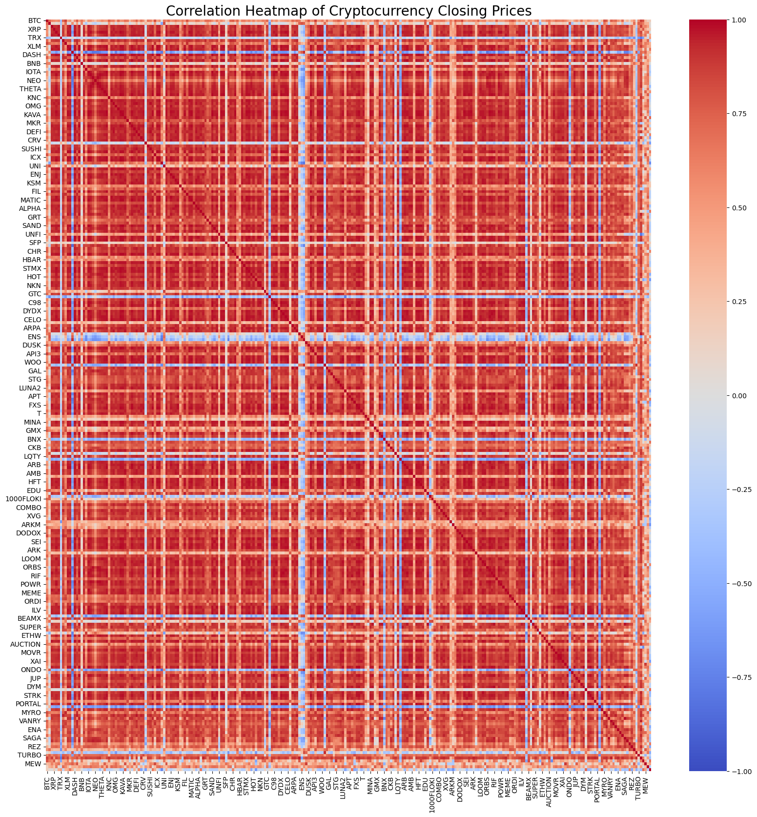
Of course, you don’t need to worry too much about how it is calculated. You can use 1 line of code in Python to calculate the correlation of all currencies. The figure shows a correlation heat map. Red represents positive correlation, blue represents negative correlation, and the darker the color, the stronger the correlation. You can see that most of the area is dark red, so the positive correlation of digital currencies is very strong.

import seaborn as sns
corr = df_close.corr()
plt.figure(figsize=(20, 20))
sns.heatmap(corr, annot=False, cmap='coolwarm', vmin=-1, vmax=1)
plt.title('Correlation Heatmap of Cryptocurrency Closing Prices', fontsize=20);

Based on the correlation, the top 20 most correlated currency pairs are selected. The results are as follows. Their correlations are very strong, all above 0.99.

MANA     SAND     0.996562
ICX      ZIL      0.996000
STORJ    FLOW     0.994193
FLOW     SXP      0.993861
STORJ    SXP      0.993822
IOTA     ZIL      0.993204
         SAND     0.993095
KAVA     SAND     0.992303
ZIL      SXP      0.992285
         SAND     0.992103
DYDX     ZIL      0.992053
DENT     REEF     0.991789
RDNT     MANTA    0.991690
STMX     STORJ    0.991222
BIGTIME  ACE      0.990987
RDNT     HOOK     0.990718
IOST     GAS      0.990643
ZIL      HOOK     0.990576
MATIC    FLOW     0.990564
MANTA    HOOK     0.990563

The corresponding code is as follows:

corr_pairs = corr.unstack()

# Remove self-correlation (i.e. values ​​on the diagonal)
corr_pairs = corr_pairs[corr_pairs != 1]

sorted_corr_pairs = corr_pairs.sort_values(kind="quicksort")

# Extract the top 20 most and least correlated currency pairs
most_correlated = sorted_corr_pairs.tail(40)[::-2]

print("The top 20 most correlated currency pairs are:")
print(most_correlated)

Backtesting Verification

The specific backtest code is as follows. The demonstration strategy mainly observes the price ratio of two cryptocurrencies (IOTA and ZIL) and trades according to the changes in this ratio. The specific steps are as follows:

1. Initialization:

• Define trading pairs (pair_a = ‘IOTA’, pair_b = ‘ZIL’).
• Create an exchange object e with an initial balance of $10,000 and a transaction fee of 0.02%.
• Calculate the initial average price ratio avg.
• Set an initial transaction value value = 1000.

2. Iterate over price data:

• Traverse the price data at each time point df_close.
• Calculates the deviation of the current price ratio from the mean diff.
• The target transaction value is calculated based on the deviation aim_value, and one value is traded for every 0.01 deviation. Buying and selling operations are determined based on the current account position and price situation.
• If the deviation is too large, execute sell pair_a and buy pair_b operations.
• If the deviation is too small, buy pair_a and sell pair_b operations are performed.

3. Adjust the mean:

• Updates the average price ratio avg to reflect the latest price ratios.

4. Update accounts and records :

• Update the position and balance information of the exchange account.
• Record the account status at each step (total assets, held assets, transaction fees, long and short positions) to res_list.

5. Result output:

• Convert res_list to dataframe res for further analysis and presentation.

pair_a = 'IOTA'
pair_b = "ZIL"
e = Exchange([pair_a,pair_b], fee=0.0002, initial_balance=10000) #Exchange definition is placed in the comments section
res_list = []
index_list = []
avg = df_close[pair_a][0] / df_close[pair_b][0]
value = 1000
for idx, row in df_close.iterrows():
    diff = (row[pair_a] / row[pair_b] - avg)/avg
    aim_value = -value * diff / 0.01
    if -aim_value + e.account[pair_a]['amount']*row[pair_a] > 0.5*value:
        e.Sell(pair_a,row[pair_a],(-aim_value + e.account[pair_a]['amount']*row[pair_a])/row[pair_a])
        e.Buy(pair_b,row[pair_b],(-aim_value - e.account[pair_b]['amount']*row[pair_b])/row[pair_b])
    if -aim_value + e.account[pair_a]['amount']*row[pair_a]  < -0.5*value:
        e.Buy(pair_a, row[pair_a],(aim_value - e.account[pair_a]['amount']*row[pair_a])/row[pair_a])
        e.Sell(pair_b, row[pair_b],(aim_value + e.account[pair_b]['amount']*row[pair_b])/row[pair_b])
    avg = 0.99*avg + 0.01*row[pair_a] / row[pair_b]
    index_list.append(idx)
    e.Update(row)
    res_list.append([e.account['USDT']['total'],e.account['USDT']['hold'],
                         e.account['USDT']['fee'],e.account['USDT']['long'],e.account['USDT']['short']])
res = pd.DataFrame(data=res_list, columns=['total','hold', 'fee', 'long', 'short'],index = index_list)
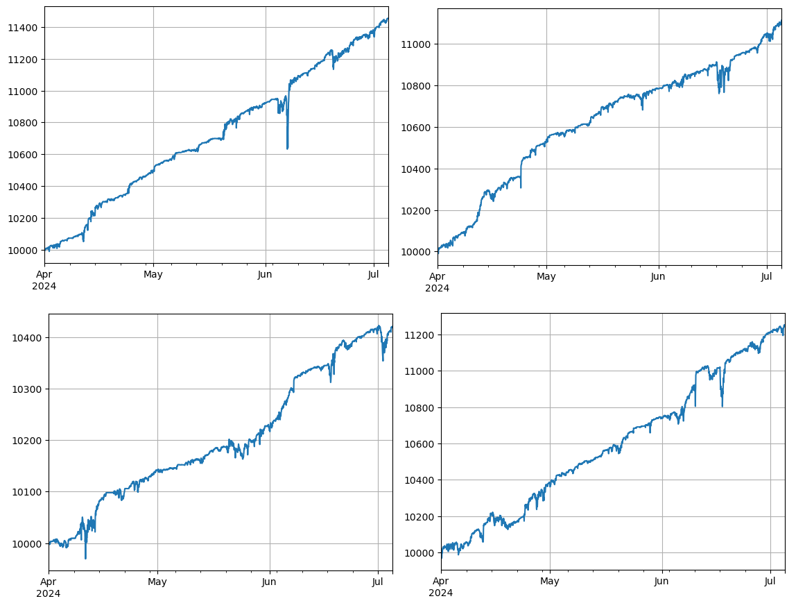
res['total'].plot(grid=True);

A total of 4 groups of currencies were backtested, and the results were ideal. The current correlation calculation uses future data, so it is not very accurate. This article also divides the data into two parts, based on the previous calculation of correlation and the subsequent backtest trading. The results are a little different but not bad. We leave it to the user to practice and verify.

Potential Risks and Ways to Improve

Although the pair trading strategy can be profitable in theory, there are still some risks in actual operation: the correlation between currencies may change over time, causing the strategy to fail; under extreme market conditions, price deviations may increase, resulting in larger losses; the low liquidity of certain currencies may make transactions difficult to execute or increase costs; and the fees generated by frequent transactions may erode profits.

To reduce risks and improve the stability of strategies, the following improvement measures can be considered: regularly recalculate the correlation between currencies and adjust trading pairs in a timely manner; set stop loss and take profit points to control the maximum loss of a single transaction; trade multiple currency pairs at the same time to diversify risks.

Conclusion

The digital currency pair trading strategy achieves profit by taking advantage of the correlation of currency prices and performing arbitrage operations when prices deviate. This strategy has high theoretical feasibility. A simple live trading strategy source code based on this strategy will be released later. If you have more questions or need further discussion, please feel free to communicate.