Measuring risk and return by the use of the Goma-Kovitz Theory
Author: The grass, Created: 2023-11-10 15:44:53, Updated: 2024-11-08 09:06:34
Last week I was introduced toVaR risk managementThe risk of a portfolio is not the same as the risk of the individual assets, and is related to their price correlation. For example, if two assets are very strongly correlated positively, i.e. if they fall into the same category, then diversification into multiple investments does not reduce the risk. If the negative correlation is strong, diversification can significantly reduce the risk.
Modern Portfolio Theory (MPT), proposed by Harry Markowitz in 1952, is a mathematical framework for portfolio selection designed to maximize expected returns while controlling risk by selecting different risky asset portfolios. The central idea is that price changes between assets that are not perfectly synchronous (i.e. that there is an imperfect correlation between assets) can reduce overall investment risk by diversifying asset allocations.
Key concepts of the Markowitz theory
-
Expected returnsThis is the expected return of an investor holding an asset or portfolio, usually based on historical earnings data.
$E(R_p) = \sum_{i=1}^{n} w_i E(R_i)$
Here, $E ((R_p) $ is the expected rate of return of the portfolio, $w_i$ is the weight of the first $i$ asset in the portfolio, and $E ((R_i) $ is the expected rate of return of the first $i$ asset.
-
Risk (i.e. volatility or standard deviation): used to measure the uncertainty of investment returns or the volatility of investments.
$\sigma_p = \sqrt{\sum_{i=1}^{n} \sum_{j=1}^{n} w_i w_j \sigma_{ij}}$
Here, $\sigma_p$ is the total risk of the portfolio, and $\sigma_{ij}$ is the reciprocal of asset $i$ and asset $j$, which measures the relationship between the price movements of these two assets.
-
Co-operationIt measures the relationship between price movements of two assets.
$\sigma_{ij} = \rho_{ij} \sigma_i \sigma_j$
Here, $\rho_{ij}$ is the coefficient of the assets $i$ and $j$, and $\sigma_i$ and $\sigma_j$ are the standard deviation of the assets $i$ and $j$, respectively.
-
Effective boundariesIn a risk-reward coordinate system, the effective boundary is the set of portfolios that can provide the maximum expected return at a given level of risk.
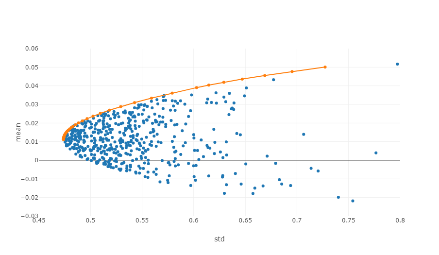
The graph above is a graph of the effective boundary, with each point representing a different weighted portfolio, with the horizontal coordinates being the volatility, or risk level, and the vertical coordinates being the yield. Obviously, we focus on the top of the graph, which has the highest returns at the same risk level.
In quantitative trading and portfolio management, applying these principles involves statistical analysis of historical data, using mathematical models to estimate the expected returns, standard deviations, and correlations of various assets. Then, optimization techniques are applied to find the optimal asset reallocation. This process often involves complex mathematical operations and a lot of computer processing, which is why quantitative analysis has become so important in the modern financial field.
Example of Python code for finding the optimal combination using the analogy
The calculation of the Markowitz optimal portfolio is a multi-step process that involves several key steps, such as data preparation, simulated portfolios, and calculation of indicators.https://plotly.com/python/v3/ipython-notebooks/markowitz-portfolio-optimization/
-
Access to market data:
- Adopted
get_dataFunctions that obtain historical price data for selected digital currencies. These are the data needed to calculate returns and risks, and they are used to build portfolios and calculate Sharpe ratios.
- Adopted
-
Calculation of returns and risks:
- Use
calculate_returns_riskThe function calculates the annualized return and annualized risk (standard deviation) of each digital currency. This is to quantify the historical performance of each asset for use in the optimal combination.
- Use
-
Calculate the optimal Makowitz combination:
- Use
calculate_optimal_portfolioFunctions that simulate multiple portfolios. In each simulation, weights of assets are randomly generated and the expected returns and risks of the portfolio are calculated based on these weights. - By randomly generating combinations of different weights, multiple possible portfolios can be explored to find the best combination. This is one of the core ideas of Makowitz's group rationality.
- Use
The goal of the whole process is to find the portfolio that offers the best expected return at a given level of risk. By simulating several possible combinations, investors can better understand the performance of different configurations and choose the combination that best suits their investment objectives and risk tolerance. This approach helps to optimize investment decisions and make investments more efficient.
import numpy as np
import pandas as pd
import requests
import matplotlib.pyplot as plt

# 获取行情数据
def get_data(symbols):
    data = []
    for symbol in symbols:
        url = 'https://api.binance.com/api/v3/klines?symbol=%s&interval=%s&limit=1000'%(symbol,'1d')
        res = requests.get(url)
        data.append([float(line[4]) for line in res.json()])
    return data

def calculate_returns_risk(data):
    returns = []
    risks = []

    for d in data:
        daily_returns = np.diff(d) / d[:-1]
        annualized_return = np.mean(daily_returns) * 365
        annualized_volatility = np.std(daily_returns) * np.sqrt(365)

        returns.append(annualized_return)
        risks.append(annualized_volatility)

    return np.array(returns), np.array(risks)

# 计算马科维茨最优组合
def calculate_optimal_portfolio(returns, risks):
    n_assets = len(returns)
    num_portfolios = 3000

    results = np.zeros((4, num_portfolios), dtype=object)


    for i in range(num_portfolios):
        weights = np.random.random(n_assets)
        weights /= np.sum(weights)

        portfolio_return = np.sum(returns * weights)
        portfolio_risk = np.sqrt(np.dot(weights.T, np.dot(np.cov(returns, rowvar=False), weights)))

        results[0, i] = portfolio_return
        results[1, i] = portfolio_risk
        results[2, i] = portfolio_return / portfolio_risk
        results[3, i] = list(weights) # 将权重转换为列表

    return results

symbols = ['BTCUSDT','ETHUSDT', 'BNBUSDT','LINKUSDT','BCHUSDT','LTCUSDT']
data = get_data(symbols)

returns, risks = calculate_returns_risk(data)
optimal_portfolios = calculate_optimal_portfolio(returns, risks)

max_sharpe_idx = np.argmax(optimal_portfolios[2])
optimal_return = optimal_portfolios[0, max_sharpe_idx]
optimal_risk = optimal_portfolios[1, max_sharpe_idx]
optimal_weights = optimal_portfolios[3, max_sharpe_idx]

# 输出结果
print("最优组合:")
for i in range(len(symbols)):
    print(f"{symbols[i]}权重: {optimal_weights[i]:.4f}")

print(f"预期收益率: {optimal_return:.4f}")
print(f"预期风险(标准差): {optimal_risk:.4f}")
print(f"夏普比率: {optimal_return / optimal_risk:.4f}")

# 可视化投资组合
plt.figure(figsize=(10, 5))
plt.scatter(optimal_portfolios[1], optimal_portfolios[0], c=optimal_portfolios[2], marker='o', s=3)
plt.title('portfolio')
plt.xlabel('std')
plt.ylabel('return')
plt.colorbar(label='sharp')
plt.show()
The final output is:
The best combination:
Weight of BTCUSDT: 0.0721
ETHUSDT weighted at 0.2704
Weight of BNBUSDT: 0.3646
LINKUSDT weighted at 0.1892
BCHUSDT weighted at 0.0829
LTCUSDT weighted at 0.0209
Expected rate of return: 0.4195
Expected risk (standard deviation): 0.1219
Sharp ratio: 3.4403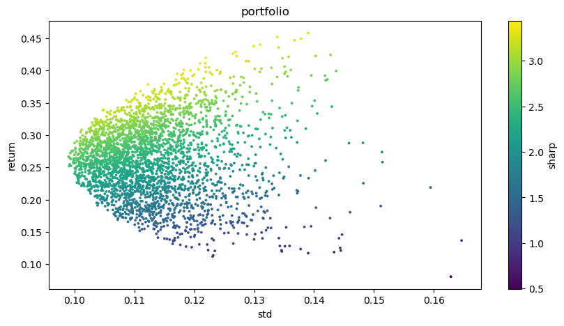
- Bayes - the mystery of decoding probability, exploring the mathematical wisdom behind decision making
- The Advantages of Using FMZ's Extended API for Efficient Group Control Management in Quantitative Trading
- Price Performance After the Currency is Listed on Perpetual Contracts
- Efficient cluster management using FMZ's extended API is an advantage in quantitative trading
- The price performance after the currency went live
- The Correlation Between the Rise and Fall of Currencies and Bitcoin
- Relation between currency declines and Bitcoin
- A Brief Discussion on the Balance of Order Books in Centralized Exchanges
- Measuring Risk and Return - An Introduction to Markowitz Theory
- Talk about the order book balance of a centralized exchange
- A Powerful Tool for Programmatic Traders: Incremental Update Algorithm for Calculating Mean and Variance
- Programmatic trader leverage: incremental update algorithm to calculate the mean and variance
- Construction and Application of Market Noise
- PSY Factor Upgrade and Transformation
- High-Frequency Trading Strategy Analysis - Penny Jump
- Alternative Trading Ideas--K-line Area Trading Strategy
- Construction and application of market noise
- PSY (psychological line) factor upgrading and transformation
- High frequency trading strategy analysis - Penny Jump
- How to Measure Position Risk - An Introduction to the VaR Method