FMEX ordering unlocked optimum to optimized quantity
Author: The grass, Created: 2020-07-03 09:30:03, Updated: 2023-09-28 21:11:27
The FMEX bankruptcy pits a lot of people, but recently came up with a restart scheme and set up rules similar to the original mining for debt relief.https://www.fmz.com/bbs-topic/5834There is also room for optimization of sort mining. Although one should not step into the same pit twice, those with credit at FMEX may want to refer to the specific real-time strategy that can run on the FMZ quantification platform.
FMEX order unlock rules
Defined as an order unlock cycle every 5 minutes of the day, each cycle allocates the trade to 1/288 of the order unlock margin for the day. Within each cycle, a randomly selected time point is taken to snapshot the ordering of the order, where:
- Buy 1 Allocates 1/4 of the return margin of the unlock cycle by the percentage of the user's ordered amount
- Selling 1 1/4 of the return margin of the order unlock cycle by user's percentage of the order volume
- Buy 2 to buy 5 of these 4 listings, divided by the user's share of the listing amount in each of the 1 listings, respectively 1/40 of the return margin of the order unlock cycle
- Sell 2 to sell 5 of these 4 listings, divided by the user's share of the amount of the listing in each 1 listing, respectively 1/40 of the return margin of the order unlock cycle
- Buy 6 to buy 10 of these 5 listings, divided by the user's share of the listing amount in each of the 1 listings, respectively 1/50 of the return margin of the order unlock cycle
- Sell 6 to sell 10 of these 5 listings, divided by the user's share of the amount of the listing in each of the 1 listings, separately divided by 1/50 of the return margin of the order unlock cycle
- Buy 11 to buy 15 of these 5 listings, divided by the user's share of the listing amount in each of the 1 listings by 1/100 of the return margin of the order unlock cycle
- Sell 11 to sell 15 of these 5 listings, divided by the user's share of the listing amount in each 1 listing, and the return margin of 1/100 of the order unlock cycle
The total return of a user's order unlock in a transaction pair on that day is the sum of the return of the user's allowance for each cycle order unlock in that transaction.
Sorting unlocks gains
The total benefits of first-order unlocking are:

where i denotes one of the positions, 30 positions on both sides, a is the order volume, R is the unlocked return amount, and V is the total number of orders already placed.
Unlike transaction unlocking, pending orders have no cost, where R only takes into account relative size and can be executed without taking into account the absolute amount of USDT billing. If we decide on the total pending order quantity, the problem becomes how to allocate the order to different locations to maximize the yield G. Simply finding the location of the smallest pending order quantity, all hanging, is obviously not optimal.
Optimized sorting unlocking
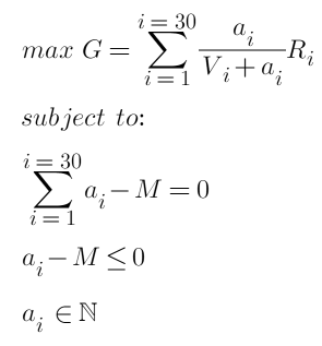
In the end, our optimization goals and constraints are:

where M is the total number of suspended units. This is a secondary convex optimization problem that contains inequalities, satisfies the KTT condition, and is solved as an integer. Using the corresponding packet and convex optimization solver should be able to directly derive the result, returning the optimal number of suspended units for each position. But this is obviously not the answer we want, we need to simplify the problem and get specific steps for solving.
Let's start with a simple example.
Considering only the case of the two classes, the current number of pending orders is 10, 20 ((referred to as the first class, second class respectively), their unlock limit is R, the total number of strategic pending orders is 30, how to allocate the funds to maximize the unlock limit?
Option one:
Find the smallest hanging position, hang all of them, and the total gain is G=30/ ((30+10) = 0.75R. This is also the easiest solution to think of.
Option two:
The first unit is assigned to the first row, the first row is assigned 10+1, and the second unit is assigned to the first row... and so on until the cumulative distribution of the first row is 10 yuan, at which point one can be randomly selected, and when the first row is more than 20, it can be assigned to the second row. The final result is that the first row is assigned 20 yuan, the second row is assigned 10 yuan, and their final list is 30.
Option three:
If the first row is assigned a, the second row is 30 - a, the equation can be directly listed as 0 (the process is not listed, similar to the article on transaction unlocking), and the final result is calculated with the formula:
G = 15 / 25 + 15 / 35 = 1.0286R, which is better than the solution 2, since it is derived directly from the formula, this is the optimal solution, the reader can verify it.
The result may be different from what is expected, and the solution 2 makes it clear that the allocation of each unit is the best in the current situation, and not the best overall. This is often the case, the local best is not necessarily the best overall, because before the allocation, the amount of the order has already been invested, and the overall efficiency needs to be taken into account.
Specific optimization
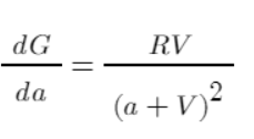
The first step is to measure the efficiency. The derivative can be used to reflect the contribution of each a to G, which takes into account the cumulative costs rather than the benefits of a single allocation. The greater the value, the greater the overall contribution to the final benefit, obviously, depending on the image of the function, a = 1, from having to zero, the highest efficiency, then gradually decreases.

The same simple example above, for example, calculates their efficiency after allocating funds, listing tables:
| Funding | 1 | 2 |
|---|---|---|
| 1 | 0.0826 | 0.0454 |
| 2 | 0.069 | 0.0413 |
| 3 | 0.0592 | 0.0378 |
| 4 | 0.051 | 0.0347 |
| 5 | 0.0444 | 0.032 |
| … | … | … |
|12 | 0.0207 |0.0195| |13 | 0.0189 |0.0184| |14 | 0.0174 |0.0173| |15 | 0.016 |0.0163| |16 | 0.0148 |0.0154| |17 | 0.0137 |0.0146| |18 | 0.0128 |0.0139|
According to the table, the 1st unit is assigned to the 1st, the 2nd unit is assigned to the 1st... the 5th unit is assigned to the 2nd... and so on, the last unit is assigned to the 1st unit is 15 yuan, the 2nd unit is 15 yuan, which happens to be the best we can calculate according to the equation.
- 1. Check all positions first, and if V = 0, then a = 1, no more excess funds will be allocated.
- 2.将总资金分配为N份,每次选择一个挡位分配。
- 3. Calculate the efficiency of each job = RV/pow ((a+V,2), where a represents the cumulative allocation of funds to the position + the current allocation of funds.
- 4.将资金分配给效率最高的挡位,效率相同随机选一个。
- 5. Cycle 3-4 until the distribution of funds is completed
If we have a large total number of hanging orders, and each unit is allocated too low in efficiency, we can divide the funds into 100 pieces, allocating one at a time, and the algorithm is very efficient because it is just a simple ordering of operations. Specific to the execution level, there is room for optimization, such as dividing our orders into 100 pieces, so that each adjustment only requires a re-allocation of the order, without removing all.
This article was originally published on FMZ's Quantitative Platform, with a footnote:https://www.fmz.com/bbs-topic-new/5843
- Introduction to the Lead-Lag suite in digital currency (3)
- Introduction to Lead-Lag Arbitrage in Cryptocurrency (2)
- Introduction to the Lead-Lag suite in the digital currency (2)
- Discussion on External Signal Reception of FMZ Platform: A Complete Solution for Receiving Signals with Built-in Http Service in Strategy
- Discussing FMZ platform external signal reception: a complete set of strategies for the reception of signals from built-in HTTP services
- Introduction to Lead-Lag Arbitrage in Cryptocurrency (1)
- Introduction to the Lead-Lag suite in digital currency (1)
- Discussion on External Signal Reception of FMZ Platform: Extended API VS Strategy Built-in HTTP Service
- External signal reception on FMZ platforms: extended API vs. built-in HTTP services
- Discussion on Strategy Testing Method Based on Random Ticker Generator
- Strategy testing methods based on random market generators explored
- Python version iceberg commission strategy
- The Logic of Crypto Currency Futures Trading
- Bottom shape ZDZB strategy
- Multi-robot market sharing solutions
- Bitcoin volatility modeling and analysis based on the ARMA-EGARCH model
- Solution of numerical calculation accuracy problem in JavaScript strategy design
- Teach you to encapsulate a Python strategy into a local file
- FMEX trading unlocks the optimal order volume optimization Part 2
- FMEX trading unlocks the optimal order volume optimization
- Analysis and Realization of Commodity Futures Volume Footprint Chart
- Calling a pin-and-pick interface to enable bot push messages
- FMEX transaction unlocked to optimized order quantity
- Simple Volatility EMV Strategy
- Handshake teaches you how to wrap a Python policy in a cost-effective document.
- Deviation rate BIAS trading strategy
- Evaluation of backtest capital curve using "pyfolio" tool
- FMZ quantified My language - interface diagram
- Python version of Commodity Futures Intertemporal Bollinger Hedge Strategy (Study purpose only)
- Interfacing with FMZ robot using "Tradingview" indicator
- FMZ Quantified My Language - Parameters of the My Language Exchange Library