Simple Trend Following Strategy
Author: ChaoZhang, Date: 2024-01-05 13:09:37Tags:

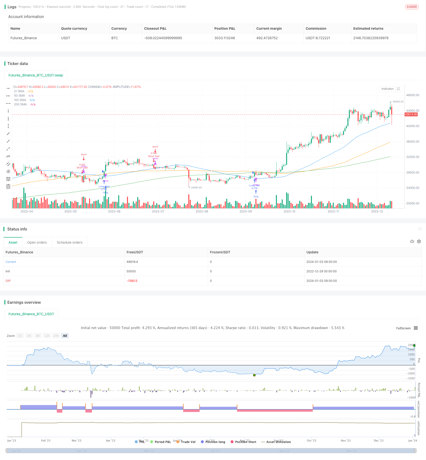
This article will analyze in detail a trend following strategy based on simple moving averages. The strategy generates trading signals using a combination of moving averages of different timeframes, belonging to a typical trend following strategy.
Strategy Overview
The strategy uses 21-day, 50-day, 100-day and 200-day simple moving averages simultaneously. It generates buy and sell signals when price breaks through these moving averages. In addition, the strategy also uses the Donchian Channel to supplement trading signals when price breaks through the 20-day or 55-day highest/lowest price. This strategy is suitable for markets with obvious trends, locking in trend profits through multiple time frames.
Strategy Principle
The core principle is to use multiple moving average time frames to determine the trend direction. Specifically, the strategy utilizes 4 simple moving averages with different time spans: 21-day, 50-day, 100-day and 200-day. The time spans of these moving averages expand gradually from short-term to long-term, used to identify trends at different levels.
When the short-term moving average crosses above the long-term one, a buy signal is generated. This indicates the market trend may have reversed and entered an uptrend. When the short-term moving average crosses below the long-term one, a sell signal is generated. This signifies the market trend may have started to reverse and enter a downtrend.
In addition, the strategy also uses the Donchian Channel to supplement trading signals. That is, when the price breaks through the 20-day or 55-day highest/lowest price, buy/sell signals will also be triggered to lock in trend profits.
In summary, the strategy combines moving average theory and Donchian Channel through multiple time frames to determine the trend direction, belonging to a typical trend following strategy.
Advantages
- Multi-timeframe design can effectively capture medium and long-term trends
- Use of both moving averages and Donchian Channel makes signals more reliable
- Simple to implement, suitable for beginners to practice quantitative trading
Risks
- Risk of false breakout. Prices may fluctuate violently for a period of time, causing incorrect signals from moving averages or Donchian Channel
- Easy to stop loss in rangy markets. The strategy is more suitable for markets with obvious trends
- Limited room for parameter optimization. It’s difficult to effectively tune parameters of moving averages and Donchian Channel
Solutions to the risks:
- Add filter conditions to avoid false breakouts, such as adding volume condition
- Appropriately reduce stop loss range to cope with rangy market
- Try introducing machine learning algorithms to auto-optimize parameters
Optimization Directions
- Add volume-based filters to avoid wrong signals during violent price fluctuations
- Try replacing moving averages with indicators that can smooth prices better, such as Kaufman’s Adaptive Moving Average
- Apply machine learning algorithms to auto-optimize parameters for better adaptation to current market conditions
- Incorporate volatility indicators to gauge trend strength, avoiding being trapped in rangy markets
Conclusion
This article has analyzed in detail a simple trend following strategy based on multi-timeframe moving averages and Donchian Channel. The strategy determines trend direction using different length moving averages, with simple and clear principles that are easy to implement. At the same time, the advantages, potential risks and future optimization ideas are also discussed. With in-depth understanding and proper optimization, I believe this strategy can become a useful tool for quantitative trading.
/*backtest
start: 2022-12-29 00:00:00
end: 2024-01-04 00:00:00
period: 1d
basePeriod: 1h
exchanges: [{"eid":"Futures_Binance","currency":"BTC_USDT"}]
*/

//@version=3
strategy("Trend Following", overlay=true, default_qty_type = strategy.percent_of_equity, default_qty_value = 10)

maxIdLossPcnt = input(1, "Max Intraday Loss(%)", type=float)
entryLong = false
entryShort = false

// strategy.risk.max_intraday_loss(maxIdLossPcnt, strategy.percent_of_equity)

if (close > highest(high[1], 20))
    strategy.entry("Long fast", strategy.long)
    entryLong = true


if (close < lowest(low[1], 20))
    strategy.entry("Short fast", strategy.short)
    entryShort = true

if (close > highest(high[1], 55))
    strategy.entry("Long slow", strategy.long)
    entryLong = true

if (close < lowest(low[1], 55))
    strategy.entry("Short slow", strategy.short)
    entryShort = true

len1 = input(21, minval=1, title="21 SMA")
src1 = input(close, title="21 SMA")
out1 = sma(src1, len1)
plot(out1, title="21 SMA", color= white)

len2 = input(50, minval=1, title="50 SMA")
src2 = input(close, title="50 SMA")
out2 = sma(src2, len2)
plot(out2, title="50 SMA", color= blue)

len3 = input(100, minval=1, title="100 SMA")
src3 = input(close, title="100 SMA")
out3 = sma(src3, len3)
plot(out3, title="100 SMA", color= orange)

len4 = input(200, minval=1, title="200 SMA")
src4 = input(close, title="200 SMA")
out4 = sma(src4, len4)
plot(out4, title="200 SMA", color= green)
- Visual Comparison between Strategy and Buy & Hold Returns
- Reversal Tracking Strategy with Double Mechanisms
- Golden Ratio Moving Average Trading Strategy
- Price Drop Buy Strategy in Downtrend with Stop Loss
- Reversal Momentum Compound Strategy
- Quantitative Trading Strategy Based on EMA Crossover
- Ichimoku Cloud Quantitative Trading Strategy
- Trend Following Moving Average Trading Strategy
- Trend Following Momentum Breakout Strategy
- Breakout and Intelligent Bollinger Bands Price Channel Strategy
- Long Breakthrough Strategy Based on K-Line Construction
- Momentum Oscillating Moving Average Trading Strategy Based on Buffered Bollinger Bands
- Adaptive Backtest Date Range Selection Strategy Based on Double MA
- Multi-Timeframe Moving Average Crossover Optimization Strategy
- Breakthrough Tracking Strategy
- Adaptive Trading Strategy Based on Momentum Indicators
- Pivot Point and Fibonacci Retracement Based Automatic Trend Following Strategy
- Trend Following Strategy Based on EMA and MACD across Timeframes
- Multi-indicator Collision Reversal Strategy
- Trend Reversal Strategy Based on EMA and SMA Crossover