Ehlers Stochastic Cyber Cycle Strategy

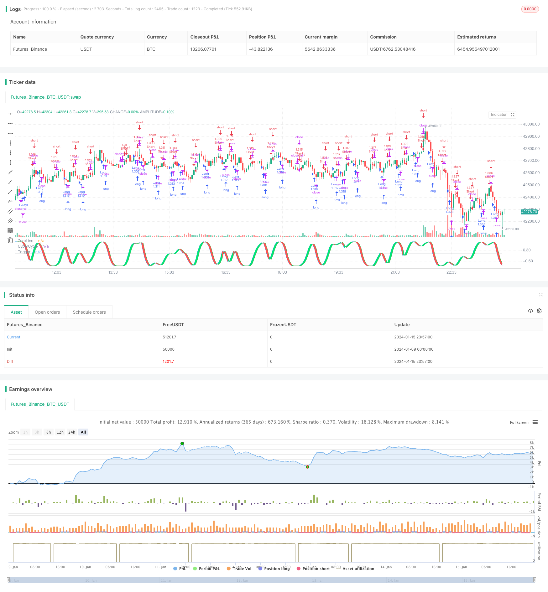
Overview

The Ehlers Stochastic Cyber Cycle Strategy is a quantitative trading strategy that generates trading signals using Ehlers’ stochastic cycle indicator. This strategy combines the advantages of stochastic indicators and cycle indicators, aiming to capture cyclical opportunities in the market.

Strategy Logic

This strategy first constructs a smoothed cycle indicator, then builds a stochastic indicator value based on that indicator. The generation of trading signals is determined by the crossover of the moving average line of this stochastic indicator value.

Specifically, the smoothed cycle indicator is calculated as:

smooth = (src + 2 * src[1] + 2 * src[2] + src[3]) / 6

Where src is the input price data, such as closing price. This indicator combines the current price and the prices of the previous 3 time periods to construct a smoothed cycle signal.

Based on this smoothed indicator, the stochastic cycle cycle can then be calculated:

cycle := (1 - .5 * alpha) * (1 - .5 * alpha) *  
           (smooth - 2 * smooth[1] + smooth[2]) +  
           2 * (1 - alpha) * cycle[1] -  
           (1 - alpha) * (1 - alpha) * cycle[2]

This calculation formula contains the second order difference of the smoothed periodic signal, and the values of the previous two cycles. α is a smoothing factor that adjusts the weight of new and old cycle values.

Finally, a 0-100 random value value1 is calculated based on this cycle indicator. And the signal value signal is constructed based on the 10-day moving average of value1. Trading signals are issued when the moving average line of signal crosses up or down.

Advantages of the Strategy

This strategy combines stochastic indicators and cycle indicators to integrate the advantages of both. Compared to simple trend strategies such as moving averages, this strategy can better capture cyclical opportunities and thus achieve better results.

The main advantages are:

1. Cycle indicators can identify cyclic patterns, stochastic indicators provide trading opportunities
2. Dual indicator design can effectively filter false signals
3. Customizable parameters suit different market environments

Risks of the Strategy

The main risks of this strategy are:

1. Improper parameter settings may lead to frequent trading, increasing trading costs and slippage costs
2. Cannot effectively handle markets with violent price fluctuations, which may lead to large losses
3. Cycle indicators rely heavily on curve fitting, improper fitting may generate wrong signals

Risks can be controlled by optimizing parameter settings, setting stop loss points, combining other filtering indicators, etc.

Optimization Directions

This strategy can also be optimized in the following aspects:

1. Combine with other technical indicators for signal filtering, such as Bollinger Bands, RSI, etc., to reduce false signals
2. Add adaptive exit mechanisms, dynamically adjust stop loss points according to market volatility
3. Use machine learning methods to automatically optimize parameters to dynamically adapt to the market
4. Optimize capital utilization through leverage, compounding and other means

Conclusion

The Ehlers Stochastic Cyber Cycle Strategy integrates the advantages of stochastic and cycle indicators through dual signal design to effectively control risks, and can achieve good returns in markets with strong cyclicality. With further optimization, this strategy can become a worthwhile quantitative trading strategy to recommend.