PINE Language Introductory Tutorial of FMZ Quant
 0
0
 3466
3466
[TOC]

PINE Language Introductory Tutorial of FMZ Quant
Supporting video tutorial: https://www.youtube.com/watch?v=CA3SwJQb_1g
FMZ Quant Trading Platform supports Pine language strategy writing, backtesting, and live trading of Pine language strategies, and it is compatible with lower versions of Pine language. There are many Pine strategies (scripts) collected and transplanted in the Strategy Square on the FMZ Quant Trading Platform (FMZ.COM).
FMZ supports not only the Pine language, but also the powerful drawing function of the Pine language. The various functions, rich and practical tools, efficient and convenient management on the FMZ platform further enhance the practicability of the Pine strategy (script). Based on the compatibility with the Pine language, FMZ also expands, optimizes and trims the Pine language to a certain extent. Before entering the tutorial officially, let’s take a look at what changes have been made to Pine language on FMZ compared to the original version.
A brief overview of some of the obvious differences:
- 1. The Pine strategy on FMZ, the version identifier at the beginning of the code
//@versionand thestrategy,indicatorstatements at the beginning of the code are not mandatory to write, FMZ does not supportimportto importlibraryfunction for now.
It may be seen that some strategies written like this:
  //@version=5
  indicator("My Script", overlay = true)
  src = close
  a = ta.sma(src, 5)
  b = ta.sma(src, 50)
  c = ta.cross(a, b)
  plot(a, color = color.blue)
  plot(b, color = color.black)
  plotshape(c, color = color.red)
Or write it like this:
  //@version=5
  strategy("My Strategy", overlay=true)

  longCondition = ta.crossover(ta.sma(close, 14), ta.sma(close, 28))
  if (longCondition)
      strategy.entry("My Long Entry Id", strategy.long)

  shortCondition = ta.crossunder(ta.sma(close, 14), ta.sma(close, 28))
  if (shortCondition)
      strategy.entry("My Short Entry Id", strategy.short)
On FMZ it can be simplified to:
  src = close
  a = ta.sma(src, 5)
  b = ta.sma(src, 50)
  c = ta.cross(a, b)
  plot(a, color = color.blue, overlay=true)
  plot(b, color = color.black, overlay=true)
  plotshape(c, color = color.red, overlay=true)
Or:
  longCondition = ta.crossover(ta.sma(close, 14), ta.sma(close, 28))
  if (longCondition)
      strategy.entry("My Long Entry Id", strategy.long)

  shortCondition = ta.crossunder(ta.sma(close, 14), ta.sma(close, 28))
  if (shortCondition)
      strategy.entry("My Short Entry Id", strategy.short)
-
- Some trading-related settings of the strategy (script) are set by the “Pine Language Trading Class Library” parameters on the FMZ strategy interface.
- Closing price model and real-time price model
On trading view, we can use the
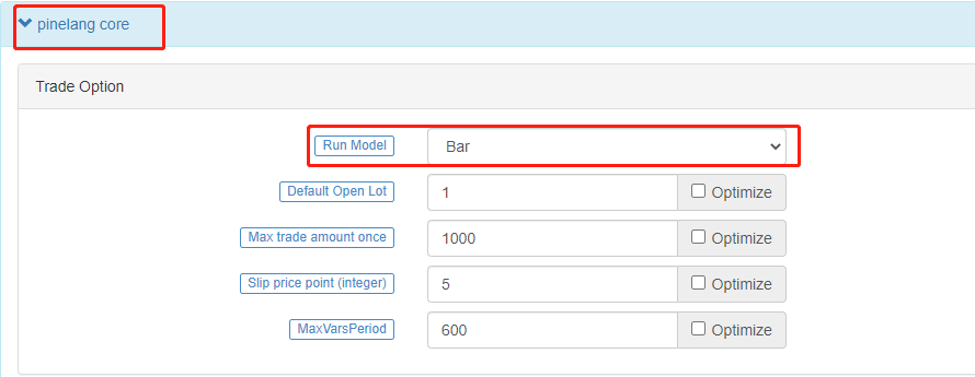
calc_on_every_tickparameter of thestrategyfunction to set the strategy script to execute the strategy logic in real time when the price changes everytime. At this time, thecalc_on_every_tickparameter should be set totrue. Thecalc_on_every_tickdefault parameter isfalse, that is, the strategy logic is executed only when the current K-line BAR of the strategy is completely completed. On FMZ, it is set by the parameters of the “Pine Language Trading Class Library” template.
Numerical precision control, such as price and order amount when the strategy is executed needs to be specified on FMZ On trading view, there is no accuracy problem when placing real trading orders, because it can only be tested in simulation. On FMZ, it is possible to run the Pine strategy in real trading. Then the strategy needs to be able to specify the price accuracy and order amount accuracy of the trading variety flexibly. The accuracy settings control the number of decimal places in the relevant data to prevent the data from not meeting the exchange’s order requirements and thus failing to place an order.
Futures contract code If the trading product on FMZ is a contract, it has two attributes, they are “Trading Pair” and “Contract Code” respectively. In addition to setting the trading pair explicitly, it is also necessary to set the specific contract code in the parameter “Variety Code” of the “Pine Language Trading Class Library” template during the real trading and backtesting. For example, for a perpetual contract, fill in
swap, and the contract code depends on whether the operating exchange has such a contract. For example, some exchanges have quarterly contracts, you can fill inquarterhere. These contract codes are consistent with the futures contract codes defined in FMZ’s Javascript/python/c++ language API document.
For other settings, such as the minimum order amount, default order amount, etc., please refer to the parameter introduction on “Template arguments of pine language trade class library” in the Pine language documentation.
- 3. Functions for FMZ extensions:
runtime.debug,runtime.log,runtime.errorused for debugging.
3 functions have been added to the FMZ platform for debugging.
runtime.debug: Print variable information on the console, which is generally not used with this function.-
```pine runtime.log(1, 2, 3, close, high, ...), Multiple parameters can be passed. -
```pine runtime.error(message) -
- The
overlayparameter is extended in some of the drawing functions
- The
In the Pine language on FMZ, the drawing functions plot, plotshape, plotchar, etc. have added the overlay parameter support, allowing to specify the drawing on the main chart or sub-chart. overlay is set to true to draw on the main chart, and false is set to draw on the sub-chart, which enables the Pine strategy on FMZ to draw the main chart and the sub-chart at the same time.
- 5. Value of the
syminfo.mintickbuilt-in variable
The built-in variable of syminfo.mintick is defined as the minimum tick value for the current symbol. This value can be controlled by the template parameter pricing currency precision in the “Pine Language Trading Class Library” on the FMZ bot/backtest interface. Pricing currency accurancy setting 2 means that the price is accurate to the second decimal place when trading, and the minimum price change unit is 0.01. The value of syminfo.mintick is 0.01.
- 6. The average price in FMZ PINE Script are all inclusive of commission
For example: the order price is 8000, the selling direction, the quantity is 1 lot (piece, sheet), the average price after the transaction is not 8000, but lower than 8000 (the cost includes the handling fee).
Pine Language Basics
When starting to learn the basics of the Pine language, there may be some examples of instructions and code grammar that we are not familiar with. It doesn’t matter if you don’t understand it, we can get familiar with the concepts first and understand the purpose of the test, or you can check the Pine language documentation on FMZ for instructions. Then follow the tutorial step by step to familiarize yourself with various grammars, instructions, functions, and built-in variables.
Model execution
When starting to learn the Pine language, it is very necessary to understand the related concepts such as the execution process of the Pine language script program. The Pine language strategy runs based on the chart. It can be understood that the Pine language strategy is a series of calculations and operations, which are executed on the chart in the order of time series from the earliest data that has been loaded on the chart. The amount of data that the chart initially loads is limited. In the real trading, the maximum amount of the data is usually determined based on the maximum data volume returned by the exchange interface, and the maximum amount of the data during backtesting is determined based on the data provided by the data source of the backtesting system. The leftmost K-line Bar on the chart, that is, the first data of the chart data set, has an index value of 0. The index value of the current K-line Bar when the Pine script is executed can be referenced through the built-in variable bar_index in the Pine language.
plot(bar_index, "bar_index")
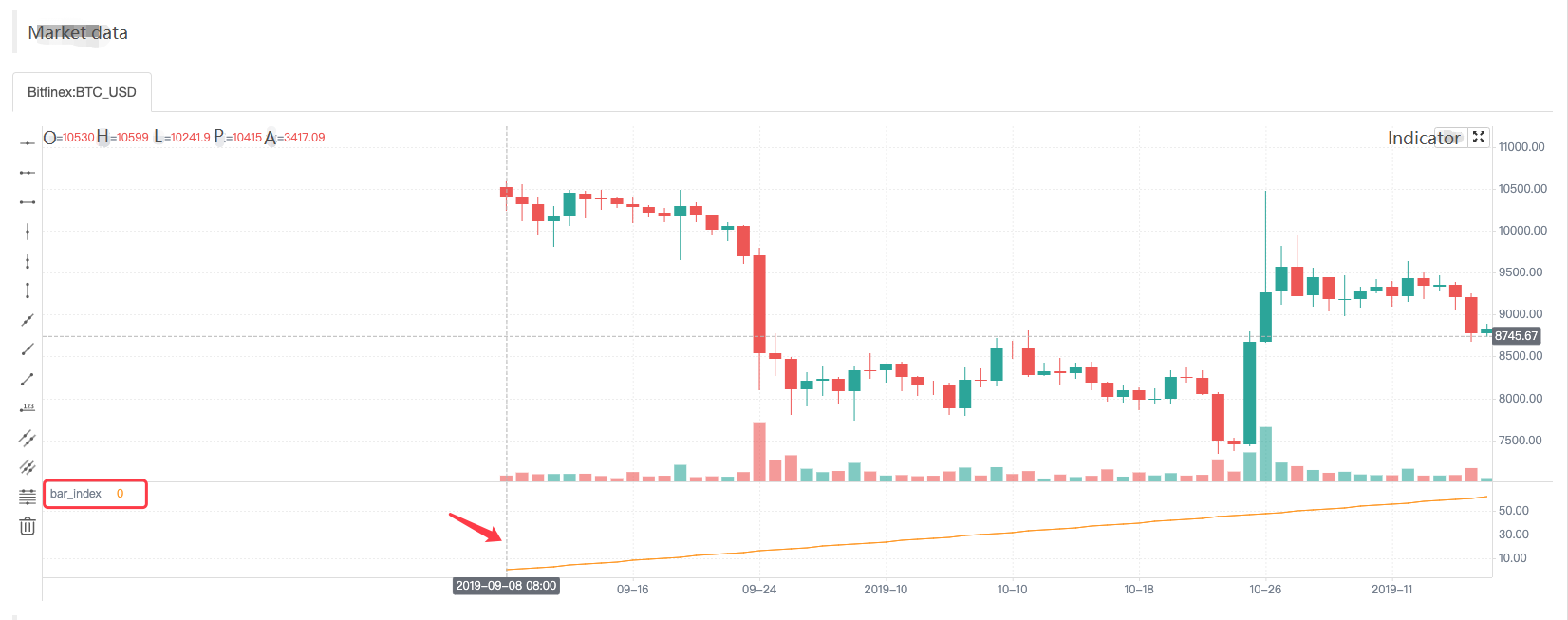
The plot function is one of the functions we will use more in the future. The use is very simple, it is to draw a line on the chart according to the input parameters, the input data is bar_index, and the line is named as bar_index. It can be seen that the value of the line named bar_index on the first Bar is 0, and it increases by 1 to the right as the Bar increases.
Because the settings of the strategy are different, the model execution methods of the strategy are different, they can be divided into closing price model and real-time price model. We have also briefly introduced the concepts of them before.
- Closing price model
When the strategy code is executed, the period of the current K-line Bar is completely executed, and when the K-line is closed, the K-line period has been completed. At this point, the Pine strategy logic is executed once, and the triggered trading signal will be executed at the beginning of the next K-line Bar.
- Real-time price model
When the strategy code is executed, regardless of whether the current K-line Bar is closed or not, the Pine strategy logic will be executed when the market changes every time, and the triggered trading signal will be executed immediately.
When the Pine language strategy is executed from left to right on the chart, the K-line Bars on the chart are divided into Historical Bars and Real-time Bars:
- Historical Bar
When the strategy is set to “Tick Model” and starts executing, all K-line Bars on the chart except the rightmost one are Historical Bars. The strategy logic is executed only once on each historical bar.
When the strategy is set to “Bar Model” and starts executing, all bars on the chart are historical bars. The strategy logic is executed only once on each historical bar.
Calculation based on historical Bars: The strategy code is executed once in the closing state of the historical bar, and then the strategy code continues to be executed in the next historical bar until all historical bars are executed once.
- Real-time Bar
When the strategy is executed to the last K-line Bar on the far right, the Bar is a real-time Bar. After the real-time bar closed, the bar becomes a passed real-time bar (becomes a historical bar). A new real-time Bar will be generated at the far right of the chart.
When the strategy is set to “Tick Model” and starts executing, the strategy logic will be executed once for each market change on real-time bar. When the strategy is set to “Bar Model” and starts executing, the real-time bar will not be displayed on the chart.
Calculation based on real-time Bar:
If the strategy is set to “Bar Model” and the chart does not display the real-time bars, the strategy code will only be executed once when the current bar closes.
If the strategy is set to “Tick Model”, the calculation on the real-time bar is completely different from the historical bar, and the strategy code will be executed once for each market change on live trading bars. For example, the built-in variables high, low, close are determined on historical Bars, and these values may change every time when the market changes on real-time Bars. Therefore, data such as indicators calculated based on these values will also change in real-time. On a real-time Bar, close always represents the current latest price, and high and low always represent the highest point and lowest point reached since the start of the current real-time bar. These built-in variables represent the final value of the real-time Bar when it was last updated.
Rollback mechanism when executing strategies on real-time Bar (real-time price model): During real-time Bar execution, resetting user-defined variables before each new iteration of the strategy is called rollback. Let’s understand the rollback mechanism with an example of the following test code.
Attention:
  /*backtest
  ...
  ..
  .
  */
The content of the package is the backtest configuration information saved in the form of code on the FMZ platform.
  /*backtest
  start: 2022-06-03 09:00:00
  end: 2022-06-08 15:00:00
  period: 1m
  basePeriod: 1m
  exchanges: [{"eid":"Bitfinex","currency":"BTC_USD"}]
  */

  var n = 0
  if not barstate.ishistory
      runtime.log("before n + 1, n:", n, " current bar_index:", bar_index)
      n := n + 1
      runtime.log("after n + 1, n:", n, " current bar_index:", bar_index)

  plot(n, title="n")
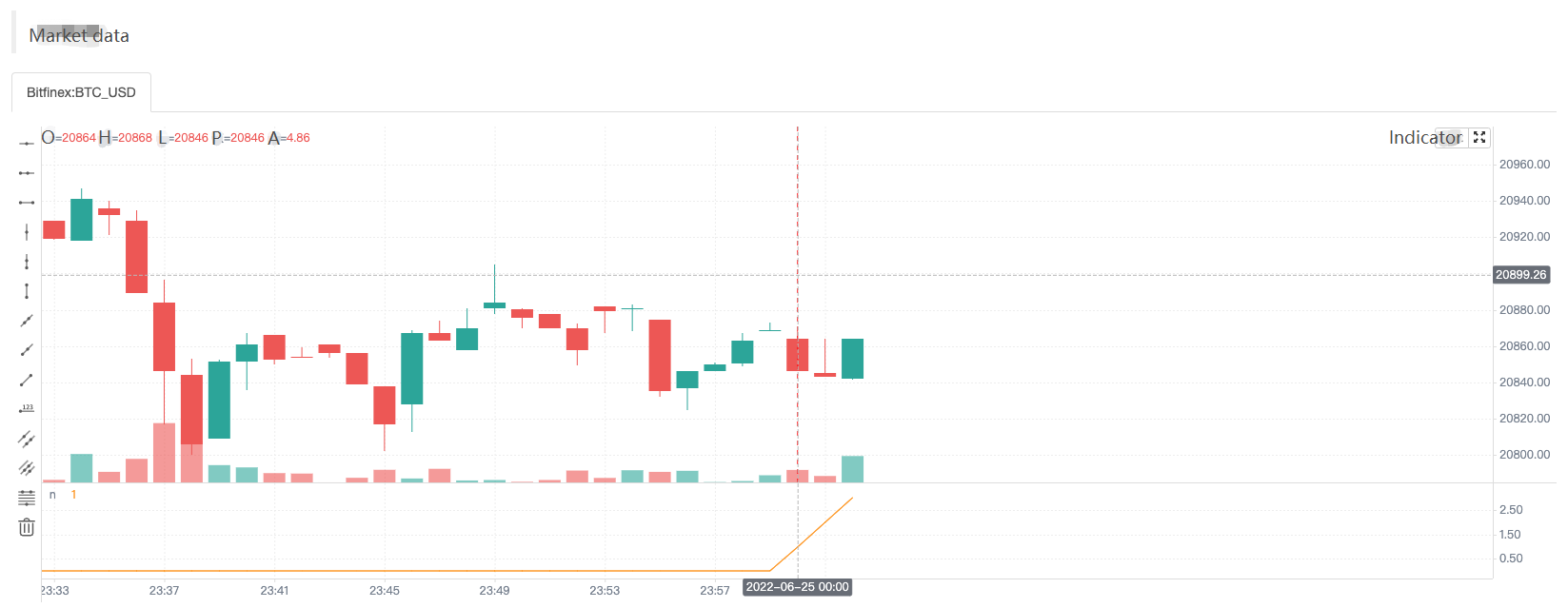
We only examine the scene executed during real-time Bars, so we use the not barstate.ishistory expression to limit the accumulation of the variable n only in the real-time Bar, and use runtime.log function to output the information in the strategy log before and after the accumulation operation. From the curve n drawn using the drawing function plot, it can be seen that n is always 0 when the strategy is running in historical Bars. When the real-time Bar is executed, the operation of adding 1 to n is triggered, and the operation of adding 1 to n is executed when the strategy is executed in each round of the real-time Bar. It can be observed from the log message that n will be reset to the value finally submitted by the previous Bar execution strategy when the strategy code is re-executed in each round. The n value update will be submitted when the strategy code is executed on the real-time Bar for the last time, so you can see that the value of curve n increases by 1 with each increase of Bar starting from the real-time Bar on the chart.
Summary: 1. The strategy code is executed once every time the market is updated when the strategy starts executing in a real-time Bar. 2. When executed in a real-time Bar, the variables are rolled back each time before the strategy code is executed. 3. When executed in a real-time Bar, the variables are submitted once when the close is updated.
Due to the data rollback, drawing operations, such as curves on the chart may also cause redrawing. For example, let’s modify the test code just now for live trading:
  var n = 0
  if not barstate.ishistory
      runtime.log("before n + 1, n:", n, " current bar_index:", bar_index)
      n := open > close ? n + 1 : n
      runtime.log("after n + 1, n:", n, " current bar_index:", bar_index)

  plot(n, title="n")
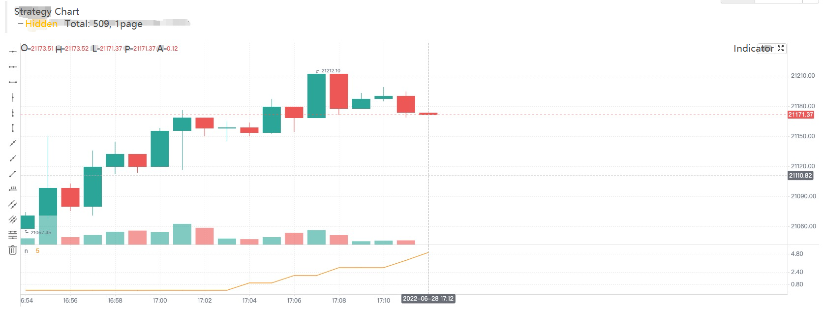
Screenshot of time A
Screenshot of time B

We only modified the sentence: n := open > close ? n + 1 : n, only add 1 to n when the current real-time Bar is a negative line (that is, the opening price is higher than the closing price). It can be seen that in the first chart (time A), since the opening price was higher than the closing price (negative line) at that time, n was accumulated by 1, and the value of n displayed on the chart curve was 5. Then the market changed and the price updated as shown in the second chart (time B). At this time, the opening price is lower than the closing price (positive line), and the n value rolls back without incrementing by 1. The curve of n in the chart is also redrawn immediately, and the value of n on the curve is 4. Therefore, the signals, such as crossup and crossdown displayed on real-time bars, are uncertain and may change.
- Variable context in functions
Let’s study the variables in the Pine language function together. According to some descriptions on Pine tutorials, the variables in the function have the following differences from the variables outside the function:
The history of series variables used in the Pine function is created with each successive call to the function. If the function is not called on every bar on which the script runs, this will result in a discrepancy between the historical values of the series inside and outside the function’s local block. Therefore, if the function is not called on each bar, the series referenced inside and outside the function with the same index value will not refer to the same historical point.
Is it a little hard to understand? Nevermind, we will figure it out with a test code running on FMZ:
  /*backtest
  start: 2022-06-03 09:00:00
  end: 2022-06-08 15:00:00
  period: 1m
  basePeriod: 1m
  exchanges: [{"eid":"Bitfinex","currency":"BTC_USD"}]
  */

  f(a) => a[1]
  f2() => close[1]

  oneBarInTwo = bar_index % 2 == 0
  plotchar(oneBarInTwo ? f(close) : na, title = "f(close)", color = color.red, location = location.absolute, style = shape.xcross, overlay = true, char = "A")
  plotchar(oneBarInTwo ? f2() : na, title = "f2()", color = color.green, location = location.absolute, style = shape.circle, overlay = true, char = "B")
  plot(close[2], title = "close[2]", color = color.red, overlay = true)
  plot(close[1], title = "close[1]", color = color.green, overlay = true)
Screenshot of backtest running
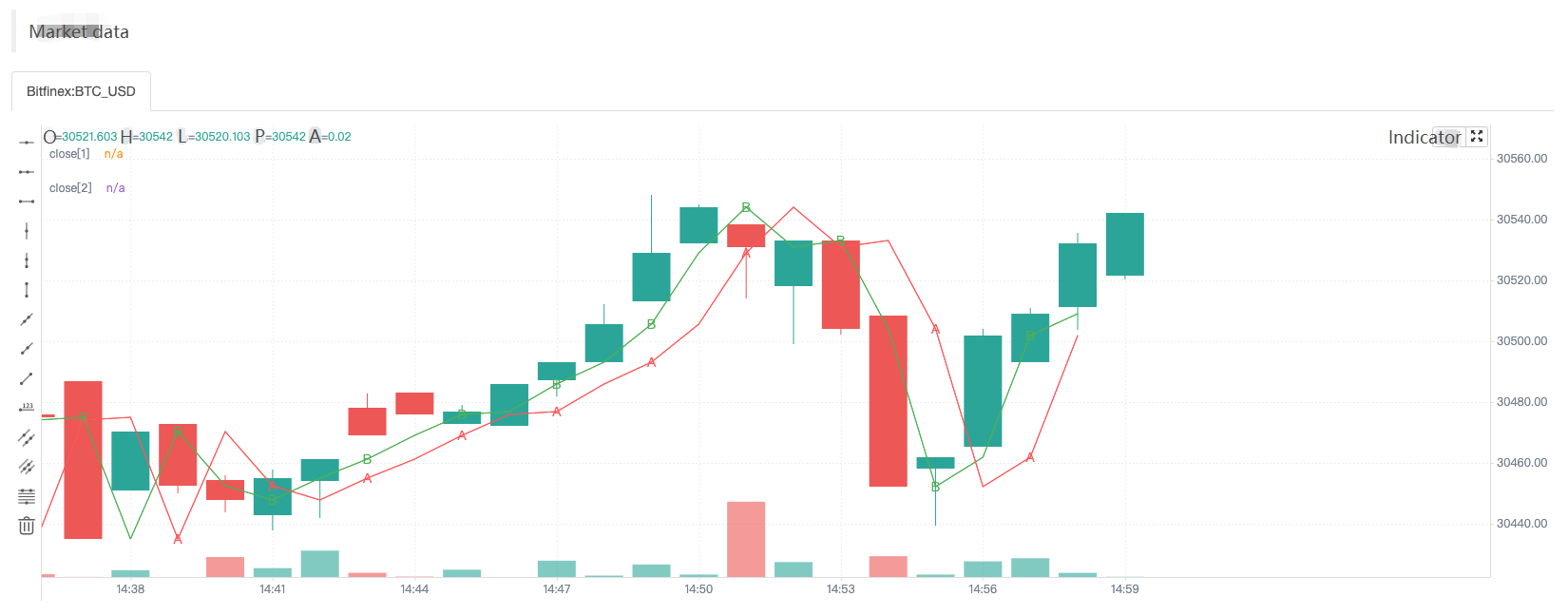
The test code is relatively simple, mainly to examine the data referenced by two methods, namely: f(a) => a[1] and f2() => close[1].
f(a) => a[1]: Use the method of passing parameters, the function returns toa[1]finally.f2() => close[1]: Use the built-in variableclosedirectly, and the function returns toclose[1]finally.
The [] symbol is used to refer to the historical value of the data series variable, and close[1] refers to the closing price data on the Bar before the current closing price. Our test code draws a total of 4 types of data on the chart:
plotchar(oneBarInTwo ? f(close) : na, title = "f(close)", color = color.red, location = location.absolute, style = shape.xcross, overlay = true, char = "A")Draw a character “A”, the color is red, it is drawn when oneBarInTwo is true, and the drawn position (on the Y axis) is: the value returned byf(close).plotchar(oneBarInTwo ? f2() : na, title = "f2()", color = color.green, location = location.absolute, style = shape.circle, overlay = true, char = "B")Draw a character “B”, the color is green, it is drawn only when oneBarInTwo is true, and the drawn position (on the Y axis) is: the value returned byf2().plot(close[2], title = "close[2]", color = color.red, overlay = true)Draw a line, the color is red, and the drawn position (on the Y-axis) is:close[2], which is the closing price of the second bar before the current bar (counting 2 bars to the left).plot(close[1], title = "close[1]", color = color.green, overlay = true)Draw a line, the color is green, and the drawn position (on the Y-axis) is:close[1], which is the closing price of the first bar before the current bar (counting 1 bar to the left).
It can be seen from the screenshot of the strategy backtesting that although both the function f(a) => a[1] used to draw the A marker and the function f2() => close[1] used to draw the B marker use [1] to refer to the historical data on the data series, the marker positions of “A” and “B” on the chart are completely different. The position of the “A” marker always falls on the red line, which is the line drawn by the code in the strategy plot(close[2], title = "close[2]", color = color.red, overlay = true), the data used to draw the line is close[2].
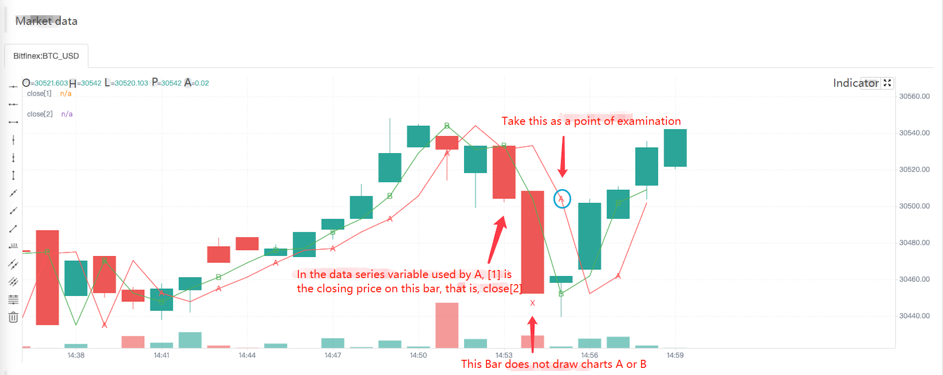
The reason is to calculate whether to draw the “A” and “B” markers through the index of the K-line Bar, that is, the built-in variable bar_index. The “A” and “B” markers are not drawn on each K-line Bar (the function calculation is called when drawing). The value referenced by the function f(a) => a[1] will not be the same as the value referenced by the function f2() => close[1] if the function is not called on every Bar (even if they both use the same index like [1]).
- Some built-in functions need to be calculated on each Bar in order to calculate their results correctly
To illustrate this situation with a simple example:
  res = close > close[1] ? ta.barssince(close < close[1]) : -1
  plot(res, style = plot.style_histogram, color=res >= 0 ? color.red : color.blue)
We write the function call code ta.barssince(close < close[1]) in a ternary operator condition ? value1 : value2. This causes the ta.barssince function to be called only when close > close[1]. But the ta.barssince function is to calculate the number of K-lines since the last time close < close[1] was established. When the ta.barssince function is called, it is always close > close[1], that is, the current closing price is greater than the closing price of the previous Bar. When the function ta.barssince is called, the condition close < close[1] is not established, and there is no recent position where it holds.
ta.barssince: When called, the function returns na if the condition has never been met before the current K-line.
As shown in the chart:
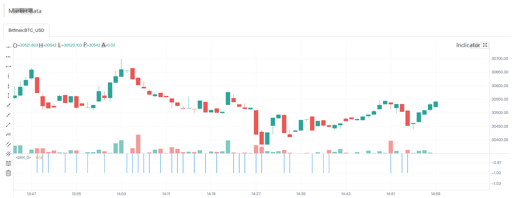
So when the chart is drawn, only the data with a value for the res variable (-1) is drawn.
To avoid this problem, we just take the ta.barssince(close < close[1]) function call out of the ternary operator and write it outside any possible conditional branches, making it perform calculations on each K-line Bar.
  a = ta.barssince(close < close[1])
  res = close > close[1] ? a : -1
  plot(res, style = plot.style_histogram, color=res >= 0 ? color.red : color.blue)
Time series
The concept of time series is very important in the Pine language, and it is a concept that we must understand when we learn the Pine language. Time series is not a type but a basic structure for storing continuous values of variables over time. We know that Pine scripts are based on charts, and the most basic content displayed in the chart is the K-line chart. Time series where each value is associated with a timestamp of a K-line Bar. open is a built-in variable (built-in) of the Pine language, and its structure is to store the time series of the opening price of each K-line Bar. It can be understood that the time series structure of open represents the opening prices of all K-line Bars from the first Bar at the beginning of the current K-line chart to the Bar where the current script is executed. If the current K-line chart is a 5-minute period, when we quote (or use) open in the Pine strategy code, it is the opening price of the K-line Bar when the strategy code is executed currently. If you want to refer to historical values in a time series, you need to use the [] operator. When the Pine strategy is executed on a certain K-line Bar, use open[1] to refer to the opening price of the previous K-line Bar (i.e., the opening price of the previous K-line period) that references the open time series on which this K-line Bar is being executed currently by the script.
- Variables on time series are very convenient for computing
Let’s take the built-in function
ta.cumas an example:
  ta.cum

  Cumulative (total) sum of `source`. In other words it's a sum of all elements of `source`.
  ta.cum(source) → series float
  RETURNS
  Total sum series.
  ARGUMENTS
  source (series int/float)
  SEE ALSO
  math.sum
Test code:
  v1 = 1
  v2 = ta.cum(v1)
  plot(v1, title="v1")
  plot(v2, title="v2")
  plot(bar_index+1, title="bar_index")
There are many built-in functions like ta.cum that can process data on time series directly. For example, ta.cum is the accumulation of the values corresponding to the variables passed in on each K-line Bar, and next we use a chart to make it easier to understand.
|Strategy operation process|Built-in variable bar_index|v1|v2| | - | - | - | - | |The strategy runs on the first K-line Bar|0|1|1| |The strategy runs on the second K-line Bar|1|1|2| |The strategy runs on the third K-line Bar|2|1|3| |…|…|…|…| |The strategy runs on the N+1th K-line Bar|N|1|N+1|
It can be seen that v1, v2 and even bar_index are all time series structures, and there is corresponding data on each bar. Whether the test code uses the “Bar model” or the “Tick model”, the only difference is whether the real-time Bar is displayed on the chart. For quick backtest, we use the “Tick model” to test.
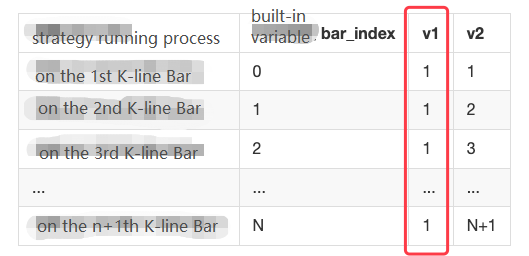
Because the variable v1 is 1 on each Bar, when the ta.cum(v1) function is executed on the first K-line Bar, there is only the first Bar, so the calculation result is 1 and assigned to variable v2.
When ta.cum(v1) is executed on the second K-line Bar, there are already 2 K-line Bars (the built-in variable bar_index corresponding to the first one is 0, and the second one corresponding to the built-in variable bar_index is 1), so the calculation result is 2, which is assigned to the variable v2, and so on. In fact, it can be observed that v2 is the number of K-line Bars in the chart, since the index of the K-line bar_index is incremented from 0, then bar_index + 1 is actually the number of K-line Bars. On the chart, we can also see that the lines v2 and bar_index do indeed overlap.
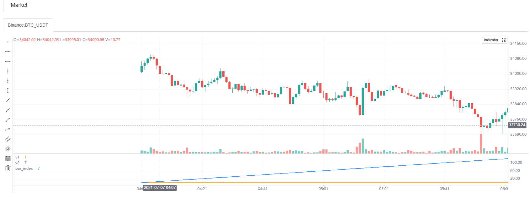
Similarly, I can also use the ta.cum built-in function to calculate the sum of the closing prices for all Bars on the current chart. All I need to do is write it like this: ta.cum(close), When the strategy runs to the real-time Bar on the far right, the result calculated by ta.cum(close) is the sum of the closing prices of all Bars on the chart (if not running to the far right, it only accumulates up to the current Bar).
Variables on the time series can also be calculated using operators, such as the code: ta.sma(high - low, 14), subtract the built-in variable high (the highest price of the K-line Bar) from low (the lowest price of K-line Bar), and finally use the ta.sma function to calculate the average value.
- The result of a function call will also leave traces of values in the time series.
  v1 = ta.highest(high, 10)[1]
  v2 = ta.highest(high[1], 10)
  plot(v1, title="v1", overlay=true)
  plot(v2, title="v2", overlay=true)
The test code runs during backtesting, and it can be observed that the values of v1 and v2 are the same, and the lines drawn on the chart are also completely coincident. The result calculated by the function call will leave traces of the value in the time series, such as the ta.highest(high, 10) in the code ta.highest(high, 10)[1]. The result calculated by the function call can also use [1] to refer to its historical value. Based on the ta.highest(high, 10) corresponding to the previous bar of the current Bar, the calculation result is ta.highest(high[1], 10). So ta.highest(high[1], 10) and ta.highest(high, 10)[1] are exactly equivalent.
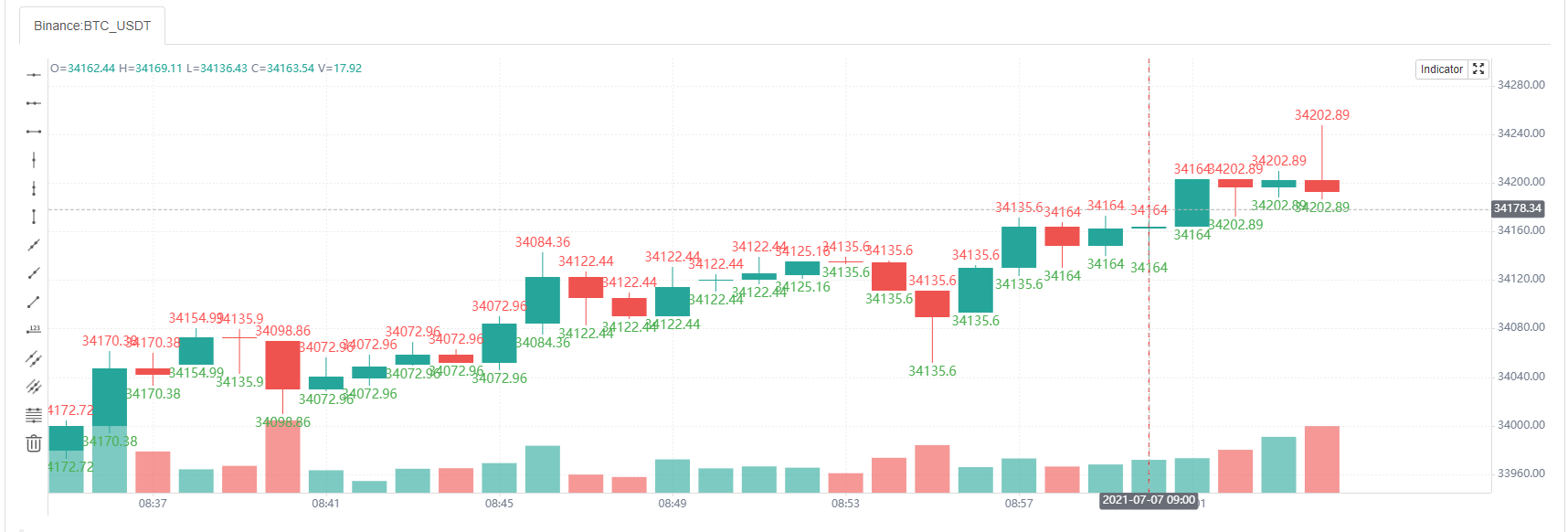
Use another drawing function to output information verification:
  a = ta.highest(close, 10)[1]
  b = ta.highest(close[1], 10)
  plotchar(true, title="a", char=str.tostring(a), location=location.abovebar, color=color.red, overlay=true)
  plotchar(true, title="b", char=str.tostring(b), location=location.belowbar, color=color.green, overlay=true)
We can see that the values of variable a and variable b in the time series are displayed above and below the corresponding Bars. We can keep this drawing code during the learning process, because we may often need to output information on the chart for observation during backtesting and experimentation.
Script structure
General structure
In the beginning part of the tutorial, we have summarized some differences in using Pine language on FMZ and Trading View. When writing Pine code on FMZ, you can omit the version number, indicator(), strategy(), and library() is currently not supported. Of course, in order to be compatible with earlier versions of Pine scripts, strategies such as: //@version=5, indicator(), strategy() can also be written. Some strategy settings can also be set by passing parameters in the strategy() function.
<version>
<declaration_statement>
<code>
The <version> version control information can be omitted.
Comments
The Pine language uses // as a single-line comment symbol, since the Pine language does not have a multi-line comment symbol. FMZ extends the comment symbol /**/ for multi-line comments.
Code
Lines in the script that are not comments or compiler directives are statements, which implement the script’s algorithm. A statement can be one of these contents.
- Variable declaration
- Reassignment of variables
- Function declaration
- Built-in function calls, user-defined function calls
if,for,whileorswitchstructure
Statements can be arranged in various ways
- Some statements can be expressed in one line, such as most variable declarations, lines containing only one function call, or single-line function declarations. Others, like structures, always require multiple lines, because they require a local block.
- Statements in the global scope of a script (i.e. parts that are not part of a local block) cannot begin with a
spaceor `tab(tab key). Their first character must also be the first character of the line. Lines starting at the first position, by definition, become part of the global scope of the script. - A structure or multi-line function declaration always requires a
local block. A local block must be indented by one tab or four spaces (otherwise, it will be parsed as the concatenated code of the previous line, that is, judged to be the continuous content of the previous line of code), and each local block defines a different local scope. - Multiple single-line statements can be concatenated in a single line by using commas (,) as separators.
- A line can contain comments or has comments only.
- Lines can also be wrapped (continued on multiple lines).
For example, it includes three local blocks, one in the custom function declaration, and two in the variable declaration using the if structure, as follows:
indicator("", "", true)             // declaration statement (global scope), can be omitted

barIsUp() =>                        // function declaration (global scope)
    close > open                    // local block (local scope)

plotColor = if barIsUp()            // variable declaration (global scope)
    color.green                     // local block (local scope)
else
    color.red                       // local block (local scope)

runtime.log("color", color = plotColor)  // Call a built-in function to output the log (global scope)
Line break code
Long lines can be split over multiple lines, or “wrapped” up. A wrapped line must be indented by any number of spaces, as long as it is not a multiple of 4 (these boundaries are used to indent local blocks).
a = open +
      high +
          low +
             close
It can be wrapped as (note that the number of spaces indented per line cannot be a multiple of 4):
a = open +
high +
low +
close
A long plot() call can be wrapped as:
close1 = request.security(syminfo.tickerid, "D", close)      // syminfo.tickerid daily level closing price data series for the current trading pair
close2 = request.security(syminfo.tickerid, "240", close)    // syminfo.tickerid 240-minute level closing price data series for the current trading pair
plot(ta.correlation(close, open, 100),                       // line-long plot() calls can be wrapped
   color = color.new(color.purple, 40),
   style = plot.style_area,
   trackprice = true)
Statements in user-defined function declarations can also be wrapped. However, since a local block must begin with an indentation in grammar (4 spaces or 1 tab), when splitting it onto the next line, the continuation of a statement must begin with more than one indentation (not equal to 4 multiples of spaces). For example:
test(c, o) =>
    ret = c > o ?
       (c > o+5000 ?
          1 :
              0):
       (c < o-5000 ?
          -1 :
              0)


a = test(close, open)
plot(a, title="a")
Markers and Operators
Markers
Before recognizing variables, we must understand the concept of “markers” first. In layman’s terms, “marker” is used as the name of function and variable (used to name variables and functions). Functions will be seen in our later tutorials, let’s learn about “markers” first.
- 1. Markers must begin with an uppercase
(A-Z)or lowercase(a-z)letter or an underscore(_)as the first character of the marker. - 2. The next character after the first character of a marker can be a letter, underscore, or a number.
- 3. The naming of markers is case-sensitive.
Such as the following named markers:
fmzVar
_fmzVar
fmz666Var
funcName
MAX_LEN
max_len
maxLen
3barsDown  // Wrong naming! It used a numeric character as the leading character of the marker
Like most programming languages, Pine language also has writing suggestions. When naming identifiers, it is generally recommended to:
- 1. All uppercase letters are used to name constants.
- 2. Use the lower camel case for other marker names.
// name variables, constants
GREEN_COLOR = #4CAF50
MAX_LOOKBACK = 100
int fastLength = 7

// name functions
zeroOne(boolValue) => boolValue ? 1 : 0
Operators
Operators are some operation symbols used in programming languages to construct expressions, and expressions are computational rules designed for certain computational purposes when we write strategies. Operators in the Pine language are classified by function as:
Assignment operators, arithmetic operators, comparison operators, logical operators, ? : ternary operators, [] historical reference operators.
Taking the arithmetic operator * as an example, it is different from the type problem caused by the return result of the Pine language operator on Trading View. The following test code is provided:
//@version=5
indicator("")
lenInput = input.int(14, "Length")
factor = year > 2020 ? 3 : 1
adjustedLength = lenInput * factor
ma = ta.ema(close, adjustedLength)  // Compilation error!
plot(ma)
When executing this script on Trading View, a compilation error will occur. The reason is that after multiplying adjustedLength = lenInput * factor, the result is series int type (series), but the second parameter of the function ta.ema does not support this type. But there are no such strict restrictions on FMZ, the above code can run normally.
Let’s take a look at the use of various operators together.
Assignment Operators
There are 2 types of assignment operators: =, :=, which we have seen in several examples at the beginning part of the tutorial.
The = operator is used to assign a value to a variable when it is initialized or declared. Variables that are initialized, declared and assigned with = will start with that value on each subsequent Bar. These are valid variable declarations:
a = close           // Use built-in variables to assign values to a
b = 10000           // Use numerical assignment
c = "test"          // Use string assignment
d = color.green     // Use color value assignment
plot(a, title="a")
plot(b, title="b")
plotchar(true, title="c", char=str.tostring(c), color=d, overlay=true)
Note that the assignment statement a = close, the variable a on each Bar is the current closing price (close) of the Bar. Other variables b, c, d are unchanged and can be tested in the backtest system on FMZ, and the results can be seen on the chart.
If we use the ```:=``` operator to assign a value to an uninitialized or declared variable, it will cause an error, for example:

```pine
a := 0
Therefore, the := assignment operator is generally used to reassign existing variables, for example:
a = close > open
b = 0
if a
    b := b + 1

plot(b)
Judging if close > open (that is, the current BAR is a positive line), the variable a is true. The code in the local block of the if statement b := b + 1 is executed, and the assignment operator := is used to reassign to b, and 1 is added. Then we use the plot function to draw the value of variable b on each BAR of the time series on the chart, and connect them into a line.
Do we think that when a positive line BAR appears, b will continue to accumulate by 1? Of course not, here we declare and initialize the variable b as 0 without using any keyword designation. This sentence b=0 is executed on each BAR, so we can see that the result of this code is to reset the b variable to 0 every time, if the variable a is true, that is, in line with close > open, then b will be incremented by 1 when the code is executed in this round, and b is 1 when the plot function draws, but b is reassigned to 0 when the code is executed in the next round. This is also the place where Pine language beginners are prone to pitfalls.
When it comes to assignment operators, we must expand on two keywords: var, varip
- var
In fact, we have seen and used this keyword in previous tutorials, but we did not discuss it in details at that time. Let’s look at the description of this keyword first:
var is a keyword used for allocating and one-time initialization of variables. In general, variable assignment grammar that does not contain the keyword var causes the variable’s value to be overwritten every time the data is updated. In contrast, when variables are assigned by using the keyword var, they can “keep state” despite data updates.
We still use this example, but we use the var keyword when assigning a value to b here.
  a = close > open
  var b = 0
  if a
      b := b + 1

  plot(b)
The var keyword allows the variable b to perform the initial assignment only, and then it will not reset b to 0 every time the strategy logic is executed, so it can be observed from the line drawn at runtime that b is the number of positive line BARs that have appeared when the current K line BAR was backtested.
Variables declared by var can be written not only in the global scope, but also in code blocks, such as this example:
  strategy(overlay=true)
  var a = close
  var b = 0.0
  var c = 0.0
  var green_bars_count = 0
  if close > open
      var x = close
      b := x
      green_bars_count := green_bars_count + 1
      if green_bars_count >= 10
          var y = close
          c := y
  plot(a, title = "a")
  plot(b, title = "b")
  plot(c, title = "c")
The variable ‘a’ holds the closing price of the first bar in the series. The variable ‘b’ holds the closing price of the first ‘green’ price bar in the series. The variable ‘c’ holds the closing price of the tenth ‘green’ bar in the series.
- varip
We see the keyword varip for the first time, we can look at the description of this keyword:
varip (var intrabar persist) is a keyword for assigning and one-time initialization of variables. It is similar to the var keyword, but variables declared with varip retain their values when real-time K-line updates.
Is it difficult to understand? It doesn’t matter, we explain it through an example, it is easy to understand.
  strategy(overlay=true)

  // test var varip
  var i = 0
  varip ii = 0

  // Print the i and ii changed in each round of the strategy logic on the chart
  plotchar(true, title="ii", char=str.tostring(ii), location=location.abovebar, color=color.red)
  plotchar(true, title="i", char=str.tostring(i), location=location.belowbar, color=color.green)

  // Increment i and ii by 1 for each round of logic execution
  i := i + 1
  ii := ii + 1
This test code has different performances on “Bar Model” and “Tick Model”:
Bar Model:
Do you remember that the strategy execution we explained earlier is divided into historical BAR stage and real-time BAR stage? In the Bar Model, the historical K-line stage, the variables i, ii declared in var, varip perform incremental operations at each round of execution of the strategy code. Therefore, it can be seen that the numbers displayed on the K-line BAR of the backtest result are incremented by 1 one by one. When the historical K-line stage ends, the real-time K-line stage begins. The variables declared by var and varip begin to undergo different changes. Because it is Bar Model, the strategy code will be executed once for each price change in a K-line BAR, i := i + 1 and ii := ii + 1 will be executed once. The difference is that ii is modified every time. Although i is modified every time, the previous value will be restored when the strategy logic is executed in the next round (remember the rollback mechanism we explained in the previous “Model Execution” chapter?), and the value of i will not be updated until the current K-line BAR is completed (that is, the previous value will not be restored when the strategy logic is executed in the next round). So it can be seen that the variable i is still increased by 1 for each BAR. But variable ii is accumulated several times for each BAR.
Tick Model: Since the Tick Model executes the strategy logic only once per K-line BAR. So in the closing price model, the variables declared by var and varip behave exactly the same in the above example incrementing by 1 for each K-line BAR during the historical K-line stage and the real-time K-line stage.
Arithmetic Operators
| Operators | Description |
|---|---|
| + | Addition |
| - | Subtraction |
| * | Multiplication |
| / | Division |
| % | Modulo |
The + and - operators can be used as binary operators or as unary operators. Other arithmetic operators can only be used as binary operators and it will report an error if it was used as unary operators.
- Both sides of the arithmetic operator are numeric type, the result is a numeric type, integer or floating point depending on the result of the operation.
- If one of the operands is a string and the operator is
+, the result of the calculation is a string, the value will be converted to the string form, and then the strings are stitched together. If it is other arithmetic operator, it will try to convert the string to a value and then carry on the operation. - If one of the operands is na, the result of the calculation is the null value–na, and it will show NaN when printed on FMZ.
a = 1 + 1
b = 1 + 1.1
c = 1 + "1.1"
d = "1" + "1.1"
e = 1 + na

runtime.log("a:", a, ", b:", b, ", c:", c, ", d:", d, ", e:", e)
// a: 2 , b: 2.1 , c: 11.1 , d: 11.1 , e: NaN
The Pine language on FMZ is a little different from the Pine language on Trading View, the Pine language on FMZ is not very strict about variable types. For example:
a = 1 * "1.1"
b = "1" / "1.1"
c = 5 % "A"

plot(a)
plot(b)
plot(c)
It works on FMZ, but it reports a type error on the Trading View. If both operands of the arithmetic operator are strings, the system converts the strings to numeric values and then calculates them. If a non-numeric string cannot be computed, the result of the system operation is a null value–na.
Comparison Operators
The comparison operators are all binary operators.
| Operators | Description |
|---|---|
| < | < |
| > | > |
| <= | <= |
| >= | >= |
| != | != |
Test example:
a = 1 > 2
b = 1 < 2
c = "1" <= 2
d = "1" >= 2
e = 1 == 1
f = 2 != 1
g = open > close
h = na > 1
i = 1 > na

runtime.log("a:", a, ", b:", b, ", c:", c, ", d:", d, ", e:", e, ", f:", f, ", g:", g, ", h:", h, ", i:", i)
// a: false , b: true , c: true , d: false , e: true , f: true , g: false , h: false , i: false
As we can see, the comparison operator is very simple to use, but this is also the operator we use the most when writing strategies. Both numeric values and built-in variables can be compared, such as close, open, etc.
As with the operator, there is a difference about Pine language between FMZ and Trading View. FMZ does not have particularly strict requirements for types, therefore, such statements d = "1" >= 2 will not report an error on FMZ, and it will be executed by converting the string to a value first and then comparing the operation. On Trading View, it will report an error.
Logical Operators
| Operators | Code Symbols | Description |
|---|---|---|
| not | not | Unary operator, not operations |
| and | and | Binary operators, and operations |
| or | or | Binary operators, or operations |
When it comes to logical operators, then we must talk about true value tables. The same as we learned in high school, here we just test and learn in our backtesting system:.
a = 1 == 1  // An expression formed by using comparison operators, the result is a Boolean value
b = 1 != 1
c = not b   // Logical not operators
d = not a   // Logical not operators

runtime.log("test the logical operator:and", "#FF0000")
runtime.log("a:", a, ", c:", c, ", a and c:", a and c)
runtime.log("a:", a, ", b:", b, ", a and b:", a and b)
runtime.log("b:", b, ", c:", c, ", b and c:", b and c)
runtime.log("d:", d, ", b:", b, ", d and b:", d and b)

runtime.log("test the logical operator:or", "#FF0000")
runtime.log("a:", a, ", c:", c, ", a or c:", a or c)
runtime.log("a:", a, ", b:", b, ", a or b:", a or b)
runtime.log("b:", b, ", c:", c, ", b or c:", b or c)
runtime.log("d:", d, ", b:", b, ", d or b:", d or b)

runtime.error("stop")
In order not to overprint messages, we throw an error with the runtime.error("stop") and make it stop after printing once. After that, we can observe the output information, and we can find that the printed content is actually the same as the true value table.
Ternary Operator
Ternary expressions using the ternary operator ? : combined with operands condition ? valueWhenConditionIsTrue : valueWhenConditionIsFalse We have also used them in the previous lessons. The so-called ternary expression, ternary operator means that there are three operands in it.
In the condition ? valueWhenConditionIsTrue : valueWhenConditionIsFalse, condition is the judgment condition. If it is true, the value of the expression is: valueWhenConditionIsTrue. If condition is false, then the value of the expression is valueWhenConditionIsFalse.
Example of a convenient demonstration, although of little practical use:
a = close > open
b = a ? "positive line" : "negative line"
c = not a ? "negative line" : "positive line"
plotchar(a, location=location.abovebar, color=color.red, char=b, overlay=true)
plotchar(not a, location=location.belowbar, color=color.green, char=c, overlay=true)
What to do if we encounter a doji? It doesn’t matter! Ternary expressions can also be nested, as we did in the previous tutorial.
a = close > open
b = a ? math.abs(close-open) > 30 ? "positive line" : "doji" : math.abs(close-open) > 30 ? "negative line" : "doji"
c = not a ? math.abs(close-open) > 30 ? "negative line" : "doji" : math.abs(close-open) > 30 ? "positive line" : "doji"
plotchar(a, location=location.abovebar, color=color.red, char=b, overlay=true)
plotchar(not a, location=location.belowbar, color=color.green, char=c, overlay=true)
In fact, it is equivalent to replacing valueWhenConditionIsTrue and valueWhenConditionIsFalse in condition ? valueWhenConditionIsTrue : valueWhenConditionIsFalse with another ternary expression.
Historical Operator
Use the historical operator [] to refer to historical values on a time series. These historical values are the values of the variable on the K-line bar before the current K-line bar when the script was running. The [] operator is used after variables, expressions, and function calls. The value in [] square brackets is the offset of the historical data we want to reference from the current K-line BAR. For example, if I want to quote the closing price of the last K-line BAR, we write it as: close[1].
We’ve seen something like this in the previous lessons:
high[10]
ta.sma(close, 10)[1]
ta.highest(high, 10)[20]
close > nz(close[1], open)
The [] operator can only be used once on the same value, so it is wrong to write it like this, and an error will be reported:
a = close[1][2] // error
Here, someone may say that the operator [] is used for series structure, it seems that series structure (series) is similar to array!
Let’s use an example to illustrate the difference between series and arrays in the Pine language.
strategy("test", overlay=true)

a = close
b = close[1]
c = b[1]

plot(a, title="a")
plot(b, title="b")
plot(c, title="c")
```pine
b = close[1]
c = b[1]
But if written separately, it will not report an error. If we understand it according to the usual array, after the assignment of b = close [1], b should be a value, but c = b[1], b can still be used to refer to the historical value again by using the history operator. It can be seen that the concept of series in the Pine language is not as simple as an array. It can be understood as the historical value on the last bar of close (assigned to b), b is also a time series structure (time series), and its h
- 关于回测手续费计算方式
- 永续合约 持仓问题
- 请教一个画线类库的问题
- 有没有月化20-30的马丁加仓思路 好用红包安排
- 一分钟k线中如何买卖在最高点
- pine script 变量值问题
- ema计算问题
- 又来新问题了,关于多币种下单
- 求助,GetDepth获取数据的时间频率等问题
- exchange.SetPrecision(2, 3) 这两个是永续交易里面的哪两个字段 起什么作用呢?
- 服务器自动更新完阿里云linux系统后 使用托管者报错
- 为啥我这下不了单啊
- 回测 币安期货 ----- 品种订阅失败 BTC_USDT_Futures_Binance
- 寻找个JS语言大神
- 请问大家币安API怎么获取单笔订单的实现盈亏呀
- 请问一个服务器可以部署多个托管者么?
- 指标库(python版)
- 趋势判断相关问题
- ETH2.0来袭,有什么致富机会?可以来套保ETH,赢分叉币糖果空投
- 求助