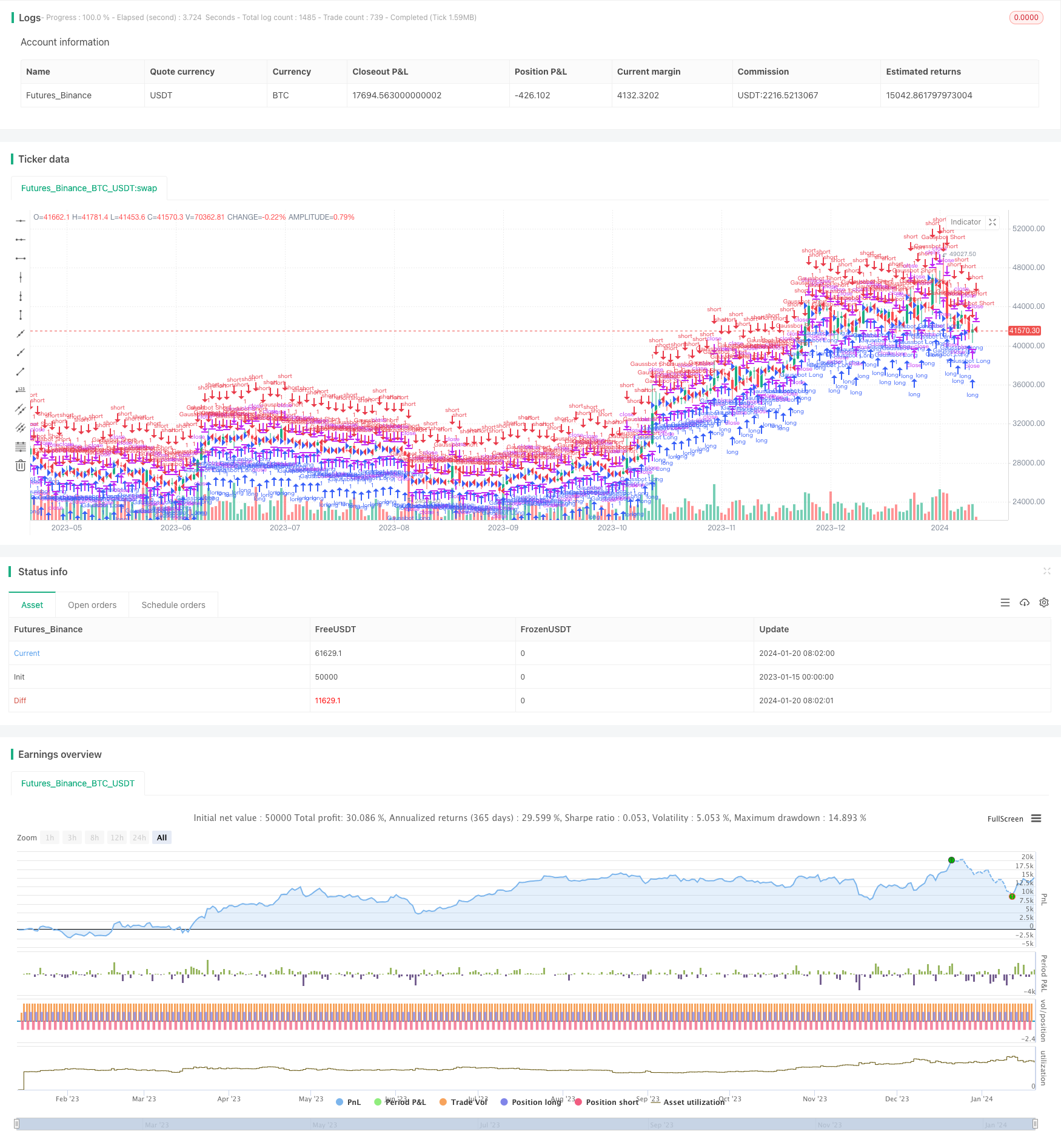
Overview
The Gauss Wave Forecasting Strategy is a quantitative trading strategy based on Gaussian filtering. It utilizes the smoothing feature of Gaussian filters to filter the price series multiple times and produce multiple smoothed price series. Then combined with polynomial fitting of these price series, it realizes the prediction of future prices. According to the prediction results, it gives suggestions on long or short positions.
Strategy Principle
The core of this strategy is the Gaussian filter algorithm. The Gaussian filter is a linear smoothing filter that uses the Gaussian function as weights. The parameter p in the strategy is set as the size of the filtering window. Then the filtering coefficient alfa is calculated through trigonometric functions. Each price series ret\[i\] represents the result after the i-th Gaussian filtering of the original price series.
The strategy employs the idea of recursion. Firstly, with alfa and the original price series price, the first filtering ret is calculated. Then based on ret, the second filtering is carried out to obtain ret2. Repeat this multiple times. Finally, by combining multiple price series, a curve is fitted to predict future prices ret4. If the predicted price is higher than the current actual price, go long. If lower than the current price, go short.
By filtering multiple times, it can be smoother and better fitting the trend. At the same time, combined with polynomial fitting, it realizes the prediction of price trends in the short term.
Advantage Analysis
The strategy has the following advantages:
Use Gaussian filter to smooth prices. It can effectively filter out high frequency noise and make the strategy more stable.
Recursive multiple filtering. It can better fit the price trend and improve the prediction effect.
Price prediction based on polynomial fitting. It can model short-term price trends and thus generate trading signals.
Judge based on current price versus predicted price. Trading signals are directly combined with trend predictions to avoid missing trading opportunities.
Simple to implement, easy to understand and optimize. It can serve as a basic module for high-frequency strategies to expand other analytical indicators.
Risk Analysis
The strategy also has the following risks:
The smoothing effect of Gaussian filter on sudden price changes may miss short-term trading opportunities.
Polynomial fitting has risks of overfitting. If the price change model mutates suddenly, the prediction effect will decline.
The size of filter window and order of fitting polynomial need to be set precisely. Otherwise it may fail.
It relies solely on opening price for trading signals and cannot trade intraday.
Optimization Directions
The strategy can be optimized in the following aspects:
Add model training and sliding window retraining mechanisms for dynamic adjustment of parameters to reduce overfitting risks.
Incorporate more price indicators and features to enrich input and make predictions more stable.
Add stop loss mechanisms, setting maximum loss ratio to avoid huge losses in extreme market conditions.
Optimize position management, dynamically adjust positions based on prediction accuracy and volatility.
Try prediction based on mainstream machine learning models like LSTM and further improve the predictive capability.
Conclusion
In summary, this is a high-frequency quantitative strategy that performs price prediction using Gaussian filter and polynomial fitting. It has certain advantages but also room for improvement. By incorporating more features, introducing dynamic parameter tuning, stop loss mechanisms etc, the strategy effect could be much better. This strategy lays the foundation as a basic module for further research and optimization of high-frequency strategies.
/*backtest
start: 2023-01-15 00:00:00
end: 2024-01-21 00:00:00
period: 1d
basePeriod: 1h
exchanges: [{"eid":"Futures_Binance","currency":"BTC_USDT"}]
*/

//@version=2
strategy("Gaussbot v1.0", overlay=true)

p = input(20, minval=1, title="Length")
price = input(open, title="Source")

pi=3.1415926535


w=2*pi/p
beta = (1 - cos(w))/(pow(1.414,2.0/3) - 1)
alfa = -beta + sqrt(beta*beta + 2*beta)
ret=  pow(alfa,4)*price+4*(1-alfa)*nz(ret[1])-6*pow(1-alfa,2)*nz(ret[2])+4*pow(1-alfa,3)*nz(ret[3])-pow(1-alfa,4)*nz(ret[4])
ret2 = pow(alfa,4)*ret+4*(1-alfa)*nz(ret2[1])-6*pow(1-alfa,2)*nz(ret2[2])+4*pow(1-alfa,3)*nz(ret2[3])-pow(1-alfa,4)*nz(ret2[4])
ret3 = pow(alfa,4)*ret2+4*(1-alfa)*nz(ret3[1])-6*pow(1-alfa,2)*nz(ret3[2])+4*pow(1-alfa,3)*nz(ret3[3])-pow(1-alfa,4)*nz(ret3[4])
ret4 = 3*ret-3*ret2+ret3


diff2 = nz(ret[1]) - nz(ret[2]) - (nz(ret[2]) - nz(ret[3]) )
diff22 = nz(ret2[1]) - nz(ret2[2]) - (nz(ret2[2]) - nz(ret2[3]) )
diff23 = nz(ret3[1]) - nz(ret3[2]) - (nz(ret3[2]) - nz(ret3[3]) )
diff24 = nz(ret4[1]) - nz(ret4[2]) - (nz(ret4[2]) - nz(ret4[3]) )


longCondition =    price[0] - ret4[1]  > 0
shortCondition =  price[0] - ret4[1] < 0

if(longCondition and shortCondition)
    longCondition = longCondition[1]
    shortCondition = shortCondition[1]
if(longCondition==false and shortCondition==false)
    longCondition = longCondition[1]
    shortCondition = shortCondition[1]


if (longCondition==true and shortCondition == false)
    strategy.entry("Gaussbot Long", strategy.long )
if (longCondition==false and shortCondition == true)
    strategy.entry("Gaussbot Short", strategy.short)