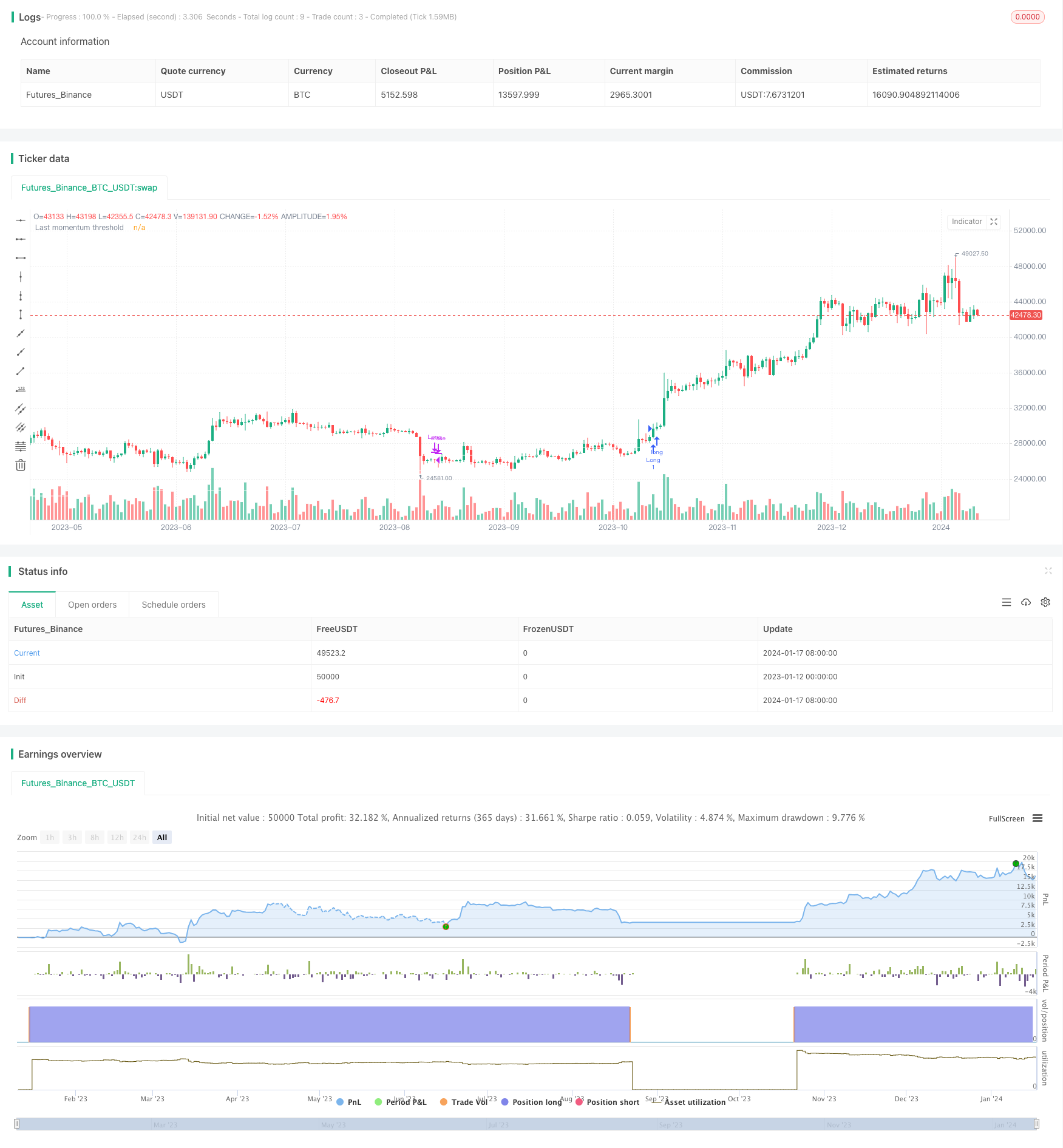
Overview
This strategy is based on the daily Heiken Ashi candlesticks, combined with momentum analysis across different timeframes, to dynamically determine the underlying support behind the current price and identify entry and exit points.
Strategy Logic
Calculate the close prices of Heiken Ashi candlesticks across different timeframes, as the basis for subsequent momentum analysis.
Calculate the percentage change between open prices and historical close prices over different periods, for both monthly and daily timeframes. This reflects the momentum strength behind the current price relative to historical levels.
Take the averages of the daily and monthly momentum fluctuations respectively. This filters out some noise and derives more stable momentum benchmarks.
Based on the average momentum fluctuations, we can calculate the market support force truly reflected by the current price, i.e. the dynamic momentum threshold exclusive of market noise.
When the close price breaks above momentum threshold, long positions are initiated on monthly basis. When price closes below threshold, positions are closed.
Pros Analysis
The biggest advantage lies in the fact that instead of simply chasing prices, the strategy calculates the real support force behind prices for entries and exits. This effectively filters out noise from ranging markets and allows us to capture stable uptrends.
Also, all underlying data is derived from Heiken Ashi candlesticks, which intrinsically helps reduce the problem of excessive reliance on linked timeframes that exists in other types of candlestick strategies. So stability is better.
Risk Analysis
The biggest risk is that momentum calculations rely solely on historical prices. If underlying company fundamentals or market regimes see significant changes, the representativeness of historical prices decreases, leading to errors in identifying entries and exits.
Also, the strategy leverages monthly and daily timeframes. This means real-time performance is not the best, lacking the ability to respond swiftly to drastic price changes. Thus there are risks of exits not triggering in time when prices suddenly turn.
Possible ways to mitigate include incorporating higher frequency data and real-time feedback on company fundamentals. Or complement with more subjective trading signals for validation and optimization.
Optimization Directions
There are a few ways in which the strategy can be further improved:
Further enhance the Heiken Ashi candles themselves i.e. optimize weight configurations.
Incorporate more timeframes, construct an exponentially averaged scoring mechanism to enhance stability.
Introduce higher frequency data such as minute bars to improve real-timeness.
Incorporate earnings warnings, M&A rumors into momentum calculations to add company fundamentals.
Consider adding day & week-based profit-taking and re-entry mechanics on top of the monthly entries.
Conclusion
In summary, the strategy is very stable over-all, with momentum tracking effectively controlling risks. The biggest advantage is using the underlying force behind prices rather than prices themselves to determine true market conditions for entries and exits. Next step is to further improve by incorporating higher frequency and more informative data to better capitalize on market opportunities.
/*backtest
start: 2023-01-12 00:00:00
end: 2024-01-18 00:00:00
period: 1d
basePeriod: 1h
exchanges: [{"eid":"Futures_Binance","currency":"BTC_USDT"}]
*/

// This Pine Script™ code is subject to the terms of the Mozilla Public License 2.0 at https://mozilla.org/MPL/2.0/
// © FrancoPassuello

//@version=5
strategy("Heiken Ashi ADM", overlay=true)
haClose = (open + high + low + close) / 4
// prevHaOpen = line.new(na, na, na, na, width = 1)
haOpen = (open[1] + close[1]) / 2
// line.set_xy1(prevHaOpen, bar_index[1], nz(haOpen[1]))
// line.set_xy2(prevHaOpen, bar_index, haClose[1])


[monopen, _1monopen, _2monopen, _3monopen, _4monopen, _5monopen, _6monopen] = request.security(syminfo.tickerid, "M", [haOpen, haOpen[1], haOpen[2], haOpen[3], haOpen[4], haOpen[5], haOpen[6]] , barmerge.gaps_off, barmerge.lookahead_on)
[monclose, _1monclose, _3monclose, _6monclose] = request.security(syminfo.tickerid, "M", [haClose, haClose[1], haClose[3], haClose[6]] , barmerge.gaps_off, barmerge.lookahead_on)
[dayclose1, _21dayclose, _63dayclose, _126dayclose, dayclose] = request.security(syminfo.tickerid, "1D", [haClose[1], haClose[21], haClose[63], haClose[126], haClose], barmerge.gaps_off, barmerge.lookahead_on)
[dayopen1, _21dayopen, _63dayopen, _126dayopen] = request.security(syminfo.tickerid, "1D", [haOpen[1], haOpen[21], haOpen[63], haOpen[126]], barmerge.gaps_off, barmerge.lookahead_on)


get_rate_of_return(price1, price2) =>
    return_ = (price1/price2 -1)*100
    return_

m0 = get_rate_of_return(monclose, monopen)
m1 = get_rate_of_return(_1monclose, _1monopen)
m2 = get_rate_of_return(monclose, _2monopen)
m3 = get_rate_of_return(_1monclose, _3monopen)
m4 = get_rate_of_return(monclose, _4monopen)
m5 = get_rate_of_return(monclose, _5monopen)
m6 = get_rate_of_return(_1monclose, _6monopen)
MS = (m1 + m3 + m6)/100
CS = (m0 + m2 + m5)/100

d1 = get_rate_of_return(dayclose1, _21dayopen)
d2 = get_rate_of_return(dayclose1, _63dayopen)
d3 = get_rate_of_return(dayclose1, _126dayopen)
DS = (d1 + d2 + d3)/100

//Last (DAILY)
lastd_s_avg1 = DS/3

lastd_Approximate1 = dayclose1*(1-lastd_s_avg1)

last_approx1_d21 = lastd_Approximate1 / _21dayopen-1
last_approx1_d63 = lastd_Approximate1 / _63dayopen-1
last_approx1_d126 = lastd_Approximate1 / _126dayopen-1

lastd_s_avg2 = (last_approx1_d21 + last_approx1_d63 + last_approx1_d126) / 3
lastd_approximate2 = (dayclose1)*(1-(lastd_s_avg1 + lastd_s_avg2))
lastd_price = lastd_approximate2

//plot(lastd_price,color = color.rgb(255, 255, 255, 14), title = "Last momentum threshold")

//Last

last_s_avg1 = MS/3

last_Approximate1 = _1monclose*(1-last_s_avg1)

last_approx1_m1 = last_Approximate1 / _1monopen-1
last_approx1_m3 = last_Approximate1 / _3monopen-1
last_approx1_m6 = last_Approximate1 / _6monopen-1

last_s_avg2 = (last_approx1_m1 + last_approx1_m3 + last_approx1_m6) / 3
last_approximate2 = (_1monclose)*(1-(last_s_avg1 + last_s_avg2))
last_price = last_approximate2
Scoring_price = _1monclose*(1-CS)

plot(last_price,color = color.rgb(255, 255, 255, 14), title = "Last momentum threshold")
//plot(Scoring_price,color = color.rgb(234, 0, 255, 14), title = "Last momentum threshold")

//Long based on month close and being the first trade of the month.

var int lastClosedMonth = -1
limit_longCondition = _1monclose > last_approximate2 and (lastClosedMonth == -1 or month(time) != lastClosedMonth)

// Long based on day close and being the first trade of the month.
limit_Dlongcondition = dayclose1 > lastd_approximate2 and (lastClosedMonth == -1 or month(time) != lastClosedMonth)

// Close trade based on day close

DCloseLongCondition = dayclose1<lastd_approximate2

//Old standard Trading rules
longCondition = _1monclose > Scoring_price
MCloseLongCondition = _1monclose<Scoring_price
shortCondition = CS < 0

if (longCondition)
    strategy.entry("Long", strategy.long)


if (strategy.position_size > 0 and MCloseLongCondition)
    strategy.close("Long")
    lastClosedMonth := month(time)