Chiến lược trọng tài thống kê thích ứng theo dõi động lượng
Tổng quan
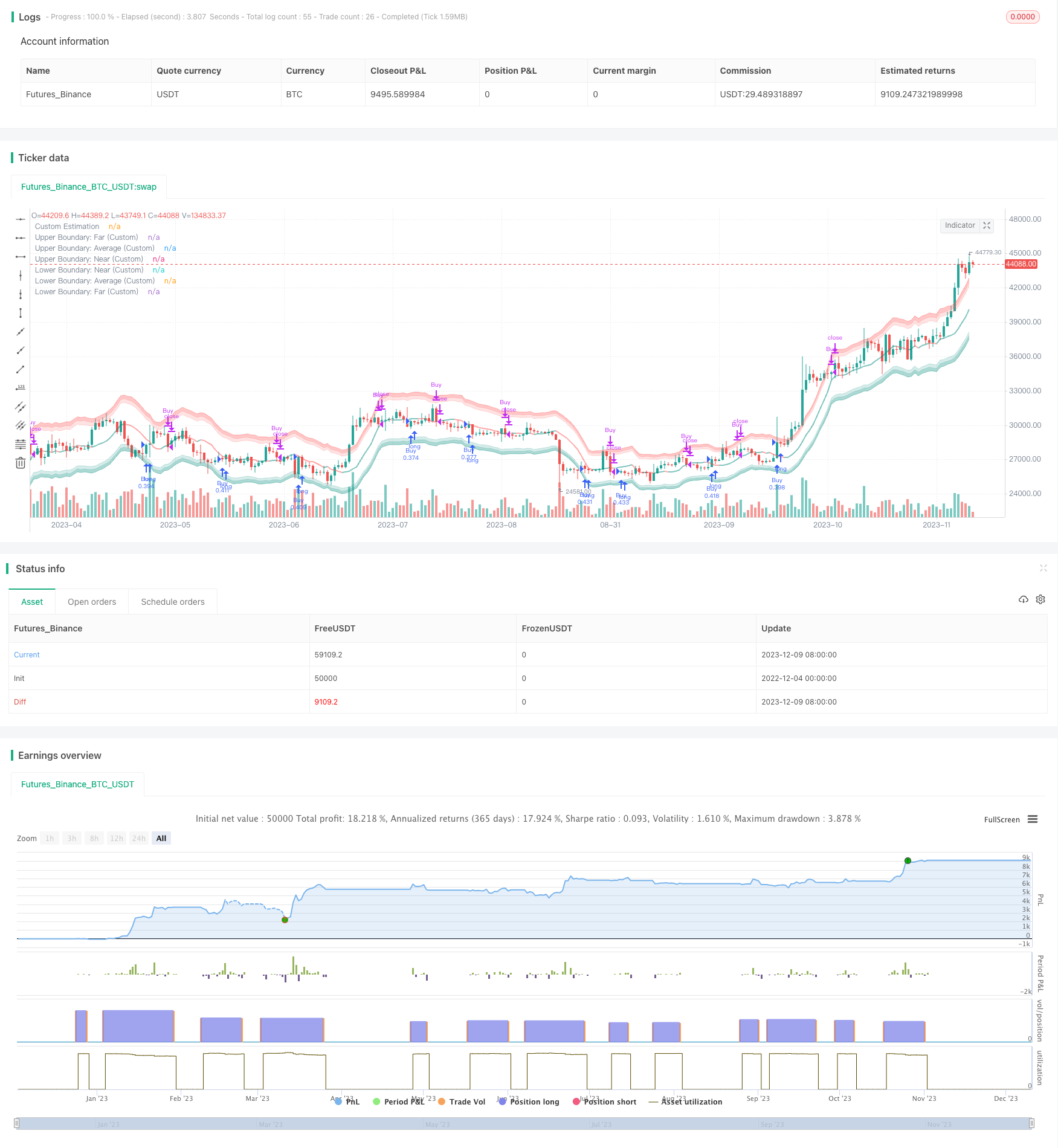
Chiến lược này dựa trên phương pháp Nadaraya-Watson Nuclear Regression để xây dựng một vòng tròn dao động động, theo dõi giá và sự giao thoa của vòng tròn, để đạt được tín hiệu giao dịch mua thấp và bán cao. Chiến lược này có cơ sở phân tích toán học và có thể thích ứng với sự thay đổi của thị trường.
Nguyên tắc chiến lược
Trọng tâm của chiến lược là tính toán các vòng tròn động của giá. Đầu tiên, dựa trên thời gian xem lại tùy chỉnh, xây dựng đường cong Nadaraya-Watson, giá ((giá đóng cửa, giá cao, giá thấp) và có được ước tính giá mịn. Sau đó, tính toán các chỉ số ATR dựa trên chiều dài ATR tùy chỉnh, kết hợp các yếu tố gần và xa để có được phạm vi của vòng tròn trên và dưới.
Lợi thế chiến lược
- Dựa trên mô hình toán học, tham số có thể điều khiển, không dễ dàng tạo ra tối ưu hóa quá mức
- Thích ứng với sự thay đổi của thị trường, nắm bắt cơ hội giao dịch bằng cách sử dụng các mối quan hệ năng động giữa giá cả và biến động
- Sử dụng tọa độ đối số, có thể xử lý tốt các giống với các chu kỳ thời gian và độ dao động khác nhau
- Tính nhạy cảm của các tham số tùy chỉnh chính sách
Rủi ro chiến lược
- Mô hình toán học lý thuyết hóa, ổ đĩa thực có thể không hoạt động như mong đợi
- Lựa chọn các tham số quan trọng cần có kinh nghiệm, thiết lập sai có thể ảnh hưởng đến thu nhập
- Có một số chậm trễ, có thể bỏ lỡ một số cơ hội giao dịch
- Những tín hiệu sai lầm có thể xảy ra trong một thị trường sụp đổ
Những rủi ro này được tránh và giảm thiểu chủ yếu bằng cách tối ưu hóa các tham số, kiểm tra lại tốt, hiểu các yếu tố ảnh hưởng và thận trọng thực tế.
Hướng tối ưu hóa chiến lược
- Tiếp tục tối ưu hóa các tham số để tìm ra sự kết hợp tham số tốt nhất
- Các tham số ưu tiên tự động sử dụng phương pháp học máy
- Thêm điều kiện lọc, kích hoạt chiến lược trong một môi trường thị trường cụ thể
- Kết hợp các chỉ số khác để lọc các tín hiệu sai lệch
- Thử các thuật toán mô hình toán học khác
Tóm tắt
Chiến lược này tích hợp phân tích thống kê và phân tích chỉ số kỹ thuật, thông qua việc theo dõi động giá và tỷ lệ biến động, để đạt được tín hiệu giao dịch mua bán thấp. Các tham số có thể được điều chỉnh tùy theo thị trường và tình hình của riêng bạn. Nói chung, nền tảng lý thuyết của chiến lược là vững chắc, hiệu suất thực tế vẫn còn cần được kiểm tra thêm.
/*backtest
start: 2022-12-04 00:00:00
end: 2023-12-10 00:00:00
period: 1d
basePeriod: 1h
exchanges: [{"eid":"Futures_Binance","currency":"BTC_USDT"}]
*/

// © Julien_Eche
//@version=5

strategy("Nadaraya-Watson Envelope Strategy", overlay=true, pyramiding=1, default_qty_type=strategy.percent_of_equity, default_qty_value=20)

// Helper Functions
getEnvelopeBounds(_atr, _nearFactor, _farFactor, _envelope) =>
    _upperFar = _envelope + _farFactor*_atr
    _upperNear = _envelope + _nearFactor*_atr
    _lowerNear = _envelope - _nearFactor*_atr
    _lowerFar = _envelope - _farFactor*_atr
    _upperAvg = (_upperFar + _upperNear) / 2
    _lowerAvg = (_lowerFar + _lowerNear) / 2
    [_upperNear, _upperFar, _upperAvg, _lowerNear, _lowerFar, _lowerAvg]

customATR(length, _high, _low, _close) =>
    trueRange = na(_high[1])? math.log(_high)-math.log(_low) : math.max(math.max(math.log(_high) - math.log(_low), math.abs(math.log(_high) - math.log(_close[1]))), math.abs(math.log(_low) - math.log(_close[1])))
    ta.rma(trueRange, length)

customKernel(x, h, alpha, x_0) =>
    sumWeights = 0.0
    sumXWeights = 0.0
    for i = 0 to h
        weight = math.pow(1 + (math.pow((x_0 - i), 2) / (2 * alpha * h * h)), -alpha)
        sumWeights := sumWeights + weight
        sumXWeights := sumXWeights + weight * x[i]
    sumXWeights / sumWeights

// Custom Settings
customLookbackWindow = input.int(8, 'Lookback Window (Custom)', group='Custom Settings')
customRelativeWeighting = input.float(8., 'Relative Weighting (Custom)', step=0.25, group='Custom Settings')
customStartRegressionBar = input.int(25, "Start Regression at Bar (Custom)", group='Custom Settings')

// Envelope Calculations
customEnvelopeClose = math.exp(customKernel(math.log(close), customLookbackWindow, customRelativeWeighting, customStartRegressionBar))
customEnvelopeHigh = math.exp(customKernel(math.log(high), customLookbackWindow, customRelativeWeighting, customStartRegressionBar))
customEnvelopeLow = math.exp(customKernel(math.log(low), customLookbackWindow, customRelativeWeighting, customStartRegressionBar))
customEnvelope = customEnvelopeClose
customATRLength = input.int(60, 'ATR Length (Custom)', minval=1, group='Custom Settings')
customATR = customATR(customATRLength, customEnvelopeHigh, customEnvelopeLow, customEnvelopeClose)
customNearATRFactor = input.float(1.5, 'Near ATR Factor (Custom)', minval=0.5, step=0.25, group='Custom Settings')
customFarATRFactor = input.float(2.0, 'Far ATR Factor (Custom)', minval=1.0, step=0.25, group='Custom Settings')
[customUpperNear, customUpperFar, customUpperAvg, customLowerNear, customLowerFar, customLowerAvg] = getEnvelopeBounds(customATR, customNearATRFactor, customFarATRFactor, math.log(customEnvelopeClose))

// Colors
customUpperBoundaryColorFar = color.new(color.red, 60)
customUpperBoundaryColorNear = color.new(color.red, 80)
customBullishEstimatorColor = color.new(color.teal, 50)
customBearishEstimatorColor = color.new(color.red, 50)
customLowerBoundaryColorNear = color.new(color.teal, 80)
customLowerBoundaryColorFar = color.new(color.teal, 60)

// Plots
customUpperBoundaryFar = plot(math.exp(customUpperFar), color=customUpperBoundaryColorFar, title='Upper Boundary: Far (Custom)')
customUpperBoundaryAvg = plot(math.exp(customUpperAvg), color=customUpperBoundaryColorNear, title='Upper Boundary: Average (Custom)')
customUpperBoundaryNear = plot(math.exp(customUpperNear), color=customUpperBoundaryColorNear, title='Upper Boundary: Near (Custom)')
customEstimationPlot = plot(customEnvelopeClose, color=customEnvelope > customEnvelope[1] ? customBullishEstimatorColor : customBearishEstimatorColor, linewidth=2, title='Custom Estimation')
customLowerBoundaryNear = plot(math.exp(customLowerNear), color=customLowerBoundaryColorNear, title='Lower Boundary: Near (Custom)')
customLowerBoundaryAvg = plot(math.exp(customLowerAvg), color=customLowerBoundaryColorNear, title='Lower Boundary: Average (Custom)')
customLowerBoundaryFar = plot(math.exp(customLowerFar), color=customLowerBoundaryColorFar, title='Lower Boundary: Far (Custom)')

// Fills
fill(customUpperBoundaryFar, customUpperBoundaryAvg, color=customUpperBoundaryColorFar, title='Upper Boundary: Farmost Region (Custom)')
fill(customUpperBoundaryNear, customUpperBoundaryAvg, color=customUpperBoundaryColorNear, title='Upper Boundary: Nearmost Region (Custom)')
fill(customLowerBoundaryNear, customLowerBoundaryAvg, color=customLowerBoundaryColorNear, title='Lower Boundary: Nearmost Region (Custom)')
fill(customLowerBoundaryFar, customLowerBoundaryAvg, color=customLowerBoundaryColorFar, title='Lower Boundary: Farmost Region (Custom)')


longCondition = ta.crossover(close, customEnvelopeLow)
if (longCondition)
    strategy.entry("Buy", strategy.long)

exitLongCondition = ta.crossover(customEnvelopeHigh, close)
if (exitLongCondition)
    strategy.close("Buy")