概述
动量方向发散策略(Momentum Direction Divergence Strategy)是一个根据威廉·布劳(William Blau)在他的书《动量,方向和发散》(Momentum, Direction and Divergence)中描述的技术之一。该策略关注三个关键方面:动量、方向和发散。布劳先生是一个电气工程师,后来成为一名交易员,他深入研究了价格和动量之间的关系。在此基础上,他分析了其他oscillator的不足,并引入了一些创新技术,包括一个新的看涨oscillator的解释。在方向性问题上,他分析了ADX的复杂性,并提供了一个独特的方法来帮助定义趋势和非趋势周期。
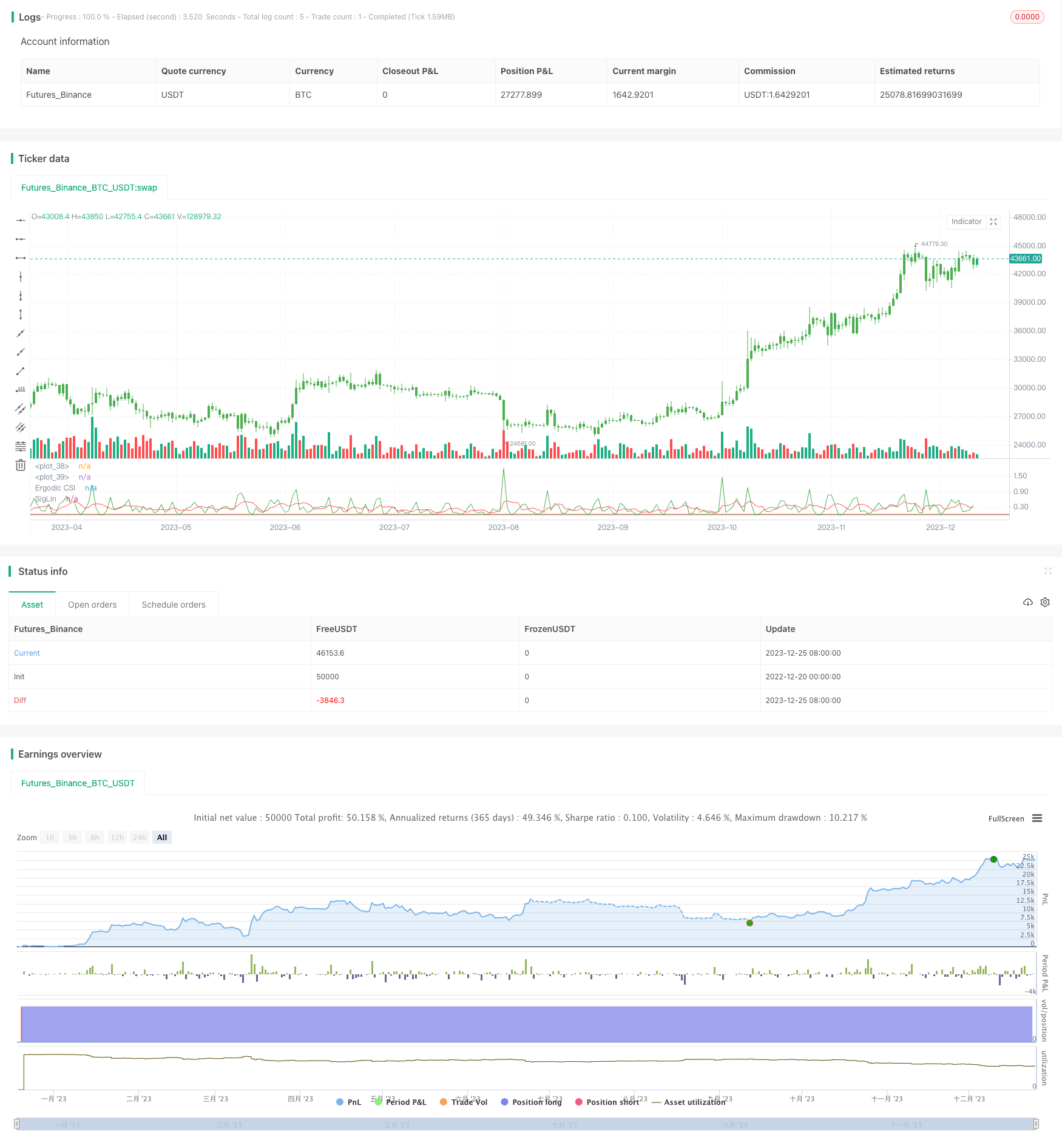
该策略绘制了动量方向发散指数(Ergotic CSI)和其平滑线,用于过滤噪音。
策略原理
代码开头定义了一个自适应动向指数(ADX)的函数fADX,它接受参数Len表示平滑周期。该函数计算真实范围(TR)的选通移动平均(RMA)作为分母,计算多头动量和空头动量的RMA作为分子,再相除得到比率,表示多头和空头的相对强度。最后通过一个公式结合多头强度和空头强度得到ADX的值。
然后是策略参数的定义。r表示ATR的平滑参数,Length表示ADX的长度,BigPointValue表示大点值,SmthLen表示平滑CSI的长度,SellZone和BuyZone表示符合条件的卖出和买入区域。reverse表示是否反转交易信号。
关键逻辑在计算CSI。首先计算真实波动幅度ATR和ADX。然后计算惩罚系数K,包含了大点值、ATR和ADX的考量。计算标准化残差nRes,它结合了ATR、ADX和收盘价的信息。最后计算CSI值,再求其平滑SMA。
根据CSI的SMA值判定交易方向。如果高于BuyZone就做多,低于SellZone就做空。绘制CSI曲线和其SMA,并用颜色标记不同的交易区间。
优势分析
该策略结合了动量指标ATR和趋势指标ADX的优点,既考虑了市场波动性,也考虑了趋势程度,避免了仅使用ATR和仅使用ADX的局限性。惩罚系数K的设计巧妙地融合了这些指标与大点值的关系。
标准化残差nRes加入了对价格信息的利用,不仅关注动量趋势,也关注价格的绝对水平,这与一般oscillator不同,增强了策略的表现力。
平滑处理和区段判断为策略决策提供了清晰的交易信号,有利于实盘操作。
风险分析
该策略对参数设置比较敏感,如ATR和ADX的周期长度,大点值的设定,CSI平滑参数等都会影响策略表现。需要通过大量回测确定合适的参数组合。
CSI作为一个新提出的oscillator,其有效性需要在更多不同市场中验证。如果该指标效果不佳,会影响策略profitability。
策略本身没有止损机制,直接按照CSI信号做多做空,存在一定程度上的风险,需要结合止损来运用。
优化方向
可以测试不同市场中的参数组合,找到一个较为通用的组合。
可以引入一个动态ADX周期长度的机制,根据市场状态来调整ADX的参数。
可以结合其他oscillator指标来决定买卖时机,使策略更加稳健。比如底部发散,顶部背离等效果。
可以加入止损策略使整体策略更加完善。
总结
动量方向发散策略整合了多种指标的优点,利用价格、动量、趋势多个维度设计CSI指标并进行交易。该策略参数设置灵活,表现力强,值得进一步测试和优化,可以成为量化交易的有利工具。
/*backtest
start: 2022-12-20 00:00:00
end: 2023-12-26 00:00:00
period: 1d
basePeriod: 1h
exchanges: [{"eid":"Futures_Binance","currency":"BTC_USDT"}]
*/

//@version=2
////////////////////////////////////////////////////////////
//  Copyright by HPotter v1.0 20/06/2018
// This is one of the techniques described by William Blau in his book
// "Momentum, Direction and Divergence" (1995). If you like to learn more,
// we advise you to read this book. His book focuses on three key aspects
// of trading: momentum, direction and divergence. Blau, who was an electrical
// engineer before becoming a trader, thoroughly examines the relationship between
// price and momentum in step-by-step examples. From this grounding, he then looks
// at the deficiencies in other oscillators and introduces some innovative techniques,
// including a fresh twist on Stochastics. On directional issues, he analyzes the
// intricacies of ADX and offers a unique approach to help define trending and
// non-trending periods.
// This indicator plots Ergotic CSI and smoothed Ergotic CSI to filter out noise.
//
// You can change long to short in the Input Settings
// WARNING:
// - For purpose educate only
// - This script to change bars colors.
////////////////////////////////////////////////////////////
fADX(Len) =>
    up = change(high)
    down = -change(low)
    trur = rma(tr, Len)
    plus = fixnan(100 * rma(up > down and up > 0 ? up : 0, Len) / trur)
    minus = fixnan(100 * rma(down > up and down > 0 ? down : 0, Len) / trur)
    sum = plus + minus
    100 * rma(abs(plus - minus) / (sum == 0 ? 1 : sum), Len)

strategy(title="Ergodic CSI Backtest")
r = input(32, minval=1)
Length = input(1, minval=1)
BigPointValue = input(1.0, minval=0.00001)
SmthLen = input(5, minval=1)
SellZone = input(0.004, minval=0.00001)
BuyZone = input(0.024, minval=0.001)
reverse = input(false, title="Trade reverse")
hline(BuyZone, color=green, linestyle=line)
hline(SellZone, color=red, linestyle=line)
source = close
K = 100 * (BigPointValue / sqrt(r) / (150 + 5))
xTrueRange = atr(1)
xADX = fADX(Length)
xADXR = (xADX + xADX[1]) * 0.5
nRes = iff(Length + xTrueRange > 0, K * xADXR * xTrueRange / Length,0)
xCSI = iff(close > 0,  nRes / close, 0)
xSMA_CSI = sma(xCSI, SmthLen)
pos = iff(xSMA_CSI > BuyZone, 1,
       iff(xSMA_CSI <= SellZone, -1, nz(pos[1], 0)))
possig = iff(reverse and pos == 1, -1,
          iff(reverse and pos == -1, 1, pos))
if (possig == 1)
    strategy.entry("Long", strategy.long)
if (possig == -1)
    strategy.entry("Short", strategy.short)
barcolor(possig == -1 ? red: possig == 1 ? green : blue )
plot(xCSI, color=green, title="Ergodic CSI")
plot(xSMA_CSI, color=red, title="SigLin")