The digital currency pairing trading strategy is detailed

The digital currency pairing trading strategy is detailed

The Preface

Recently, the quantitative diary of the BoE mentioned that it is possible to use negative correlation coins to make a profit based on price gap breakouts. Digital currencies are basically positive correlation, negative correlation is a small number of currencies, often with special markets, such as the independent market of MEME coins of the past period, completely do not follow the trend of the big disc, filter out these coins, break out and do more, this way can be profitable under certain circumstances.

Cryptocurrency pairing is a trading strategy based on statistical profit, whereby two highly correlated digital currency perpetual contracts are bought and sold at the same time in order to profit from price deviations. This article details the principles of the strategy, the profit mechanism, the method of filtering the coin species, the potential risks and how to improve it, and provides some practical Python code examples.

The Principles of Strategy

Pairing trading strategies rely on historical correlation between the prices of two digital currencies. When the prices of two currencies are strongly correlated, their price movements are largely synchronous. If the price ratios of the two appear to deviate significantly at a certain moment, it can be considered a temporary anomaly, with prices tending to return to normal. The digital currency market has a high degree of interconnectivity, and when one major digital currency (such as Bitcoin) experiences significant fluctuations, it usually triggers the interconnectivity of other digital currencies.

Assume that A and B have a higher price correlation. At a certain point in time, the average value of the A/B price ratio is 1. If at a certain point in time, the A/B price ratio deviates more than 0.001, that is, more than 1.001, then the transaction can be done as follows: open more B, open more A. Conversely, when the A/B price ratio is less than 0.999, open more A, open more B.

The key to profitability is the difference gain when the price deviates back to normal. Since the price deviation is usually short-lived, traders can break even when the price returns to the mean and profit from it, earning the difference.

Prepared data

Introducing the appropriate library

These codes can be used directly, preferably by downloading an Anancoda and debugging it in a Jupyer notebook.

import requests
from datetime import date,datetime
import time
import pandas as pd
import numpy as np
import matplotlib.pyplot as plt
import requests, zipfile, io
%matplotlib inline

Get all the trading pairs that are being traded

Info = requests.get('https://fapi.binance.com/fapi/v1/exchangeInfo')
b_symbols = [s['symbol'] for s in Info.json()['symbols'] if s['contractType'] == 'PERPETUAL' and s['status'] == 'TRADING' and s['quoteAsset'] == 'USDT']
b_symbols = list(filter(lambda x: x[-4:] == 'USDT', [s.split('_')[0] for s in b_symbols]))
b_symbols = [x[:-4] for x in b_symbols]
print(b_symbols) # 获取所有的正在交易的交易对

The function to download the K-line

The main function of the GetKlines function is to retrieve historical K-line data from the Binance exchange for specified trades on perpetual contracts and store this data in a Pandas DataFrame. The K-line data includes information such as opening price, maximum price, minimum price, closing price, volume of trades.

def GetKlines(symbol='BTCUSDT',start='2020-8-10',end='2024-7-01',period='1h',base='fapi',v = 'v1'):
    Klines = []
    start_time = int(time.mktime(datetime.strptime(start, "%Y-%m-%d").timetuple()))*1000 + 8*60*60*1000
    end_time =  min(int(time.mktime(datetime.strptime(end, "%Y-%m-%d").timetuple()))*1000 + 8*60*60*1000,time.time()*1000)
    intervel_map = {'m':60*1000,'h':60*60*1000,'d':24*60*60*1000}
    while start_time < end_time:
        time.sleep(0.3)
        mid_time = start_time+1000*int(period[:-1])*intervel_map[period[-1]]
        url = 'https://'+base+'.binance.com/'+base+'/'+v+'/klines?symbol=%s&interval=%s&startTime=%s&endTime=%s&limit=1000'%(symbol,period,start_time,mid_time)
        res = requests.get(url)
        res_list = res.json()
        if type(res_list) == list and len(res_list) > 0:
            start_time = res_list[-1][0]+int(period[:-1])*intervel_map[period[-1]]
            Klines += res_list
        if type(res_list) == list and len(res_list) == 0:
            start_time = start_time+1000*int(period[:-1])*intervel_map[period[-1]]
        if mid_time >= end_time:
            break
    df = pd.DataFrame(Klines,columns=['time','open','high','low','close','amount','end_time','volume','count','buy_amount','buy_volume','null']).astype('float')
    df.index = pd.to_datetime(df.time,unit='ms')
    return df

Downloading data

The data volume is relatively large, and only the latest 3 months of K-line data are obtained for faster downloads.

start_date = '2024-04-01'
end_date   = '2024-07-05'
period = '1h'
df_dict = {}

for symbol in b_symbols:   
    print(symbol)
    if symbol in df_dict.keys():
        continue
    df_s = GetKlines(symbol=symbol+'USDT',start=start_date,end=end_date,period=period)
    if not df_s.empty:
        df_dict[symbol] = df_s
df_close = pd.DataFrame(index=pd.date_range(start=start_date, end=end_date, freq=period),columns=df_dict.keys())
for symbol in symbols:
    df_close[symbol] = df_dict[symbol].close
df_close = df_close.dropna(how='all')

The retest engine

Defines an Exchange object for the next retest

class Exchange:
    def __init__(self, trade_symbols, fee=0.0002, initial_balance=10000):
        self.initial_balance = initial_balance #初始的资产
        self.fee = fee
        self.trade_symbols = trade_symbols
        self.account = {'USDT':{'realised_profit':0, 'unrealised_profit':0, 'total':initial_balance,
                                'fee':0, 'leverage':0, 'hold':0, 'long':0, 'short':0}}
        for symbol in trade_symbols:
            self.account[symbol] = {'amount':0, 'hold_price':0, 'value':0, 'price':0, 'realised_profit':0,'unrealised_profit':0,'fee':0}
            
    def Trade(self, symbol, direction, price, amount):
        cover_amount = 0 if direction*self.account[symbol]['amount'] >=0 else min(abs(self.account[symbol]['amount']), amount)
        open_amount = amount - cover_amount
        self.account['USDT']['realised_profit'] -= price*amount*self.fee #扣除手续费
        self.account['USDT']['fee'] += price*amount*self.fee
        self.account[symbol]['fee'] += price*amount*self.fee
        if cover_amount > 0: #先平仓
            self.account['USDT']['realised_profit'] += -direction*(price - self.account[symbol]['hold_price'])*cover_amount  #利润
            self.account[symbol]['realised_profit'] += -direction*(price - self.account[symbol]['hold_price'])*cover_amount
            self.account[symbol]['amount'] -= -direction*cover_amount
            self.account[symbol]['hold_price'] = 0 if self.account[symbol]['amount'] == 0 else self.account[symbol]['hold_price']
        if open_amount > 0:
            total_cost = self.account[symbol]['hold_price']*direction*self.account[symbol]['amount'] + price*open_amount
            total_amount = direction*self.account[symbol]['amount']+open_amount
            
            self.account[symbol]['hold_price'] = total_cost/total_amount
            self.account[symbol]['amount'] += direction*open_amount      
    
    def Buy(self, symbol, price, amount):
        self.Trade(symbol, 1, price, amount)
        
    def Sell(self, symbol, price, amount):
        self.Trade(symbol, -1, price, amount)
        
    def Update(self, close_price): #对资产进行更新
        self.account['USDT']['unrealised_profit'] = 0
        self.account['USDT']['hold'] = 0
        self.account['USDT']['long'] = 0
        self.account['USDT']['short'] = 0
        for symbol in self.trade_symbols:
            if not np.isnan(close_price[symbol]):
                self.account[symbol]['unrealised_profit'] = (close_price[symbol] - self.account[symbol]['hold_price'])*self.account[symbol]['amount']
                self.account[symbol]['price'] = close_price[symbol]
                self.account[symbol]['value'] = self.account[symbol]['amount']*close_price[symbol]
                if self.account[symbol]['amount'] > 0:
                    self.account['USDT']['long'] += self.account[symbol]['value']
                if self.account[symbol]['amount'] < 0:
                    self.account['USDT']['short'] += self.account[symbol]['value']
                self.account['USDT']['hold'] += abs(self.account[symbol]['value'])
                self.account['USDT']['unrealised_profit'] += self.account[symbol]['unrealised_profit']
        self.account['USDT']['total'] = round(self.account['USDT']['realised_profit'] + self.initial_balance + self.account['USDT']['unrealised_profit'],6)
        self.account['USDT']['leverage'] = round(self.account['USDT']['hold']/self.account['USDT']['total'],3)

Relevance analysis to screen for currency

Relativity calculus is a method in statistics used to measure the linear relationship between two variables. The most commonly used correlational calculus method is the Pearson correlation coefficient. The following are the principles, formulas, and implementations of correlational calculus. Pearson correlation coefficients are used to measure the linear relationship between two variables, taking values in the range from -1 to 1:

• 1Indicates that the two variables are always in synchronous change. When one variable increases, the other variable increases proportionally. The closer one is to one, the stronger the correlation.
• -1This means that the two variables are always inversely related. The closer to -1 the stronger the negative correlation.
• 0Indicates wireless correlation, no linear relationship between the two variables.

The Pearson correlation coefficient is determined by calculating the covariance and standard deviation of the two variables. The formula is as follows:

[ \rho_{X,Y} = \frac{\text{cov}(X,Y)}{\sigma_X \sigma_Y} ]

Some of them are:

• ( \rho_{X,Y}) is the Pearson coefficient of the variables (X) and (Y).
• (\text{cov}(X,Y) is the covariance of (X) and (Y).
• (\sigma_X) and (\sigma_Y) are the standard deviations of (X) and (Y), respectively.

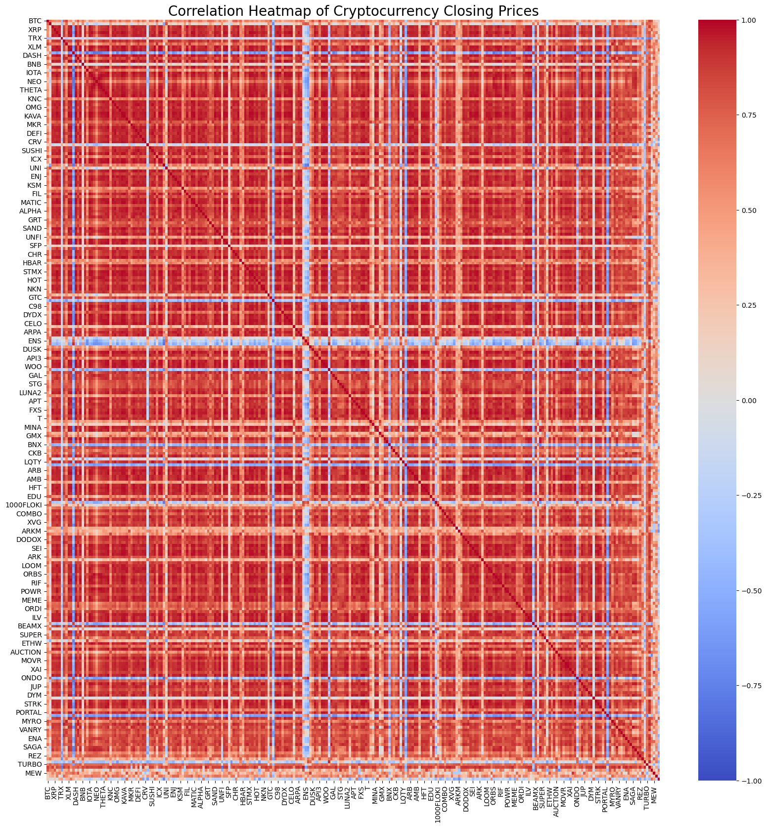
Of course, no matter how it is calculated, you can calculate the correlation of all the currencies using Python 1 line of code. The diagram shows the correlation heat graph, the red representation is positive correlation, the blue representation is negative correlation, the deeper the correlation, the stronger the correlation.

import seaborn as sns
corr = df_close.corr()
plt.figure(figsize=(20, 20))
sns.heatmap(corr, annot=False, cmap='coolwarm', vmin=-1, vmax=1)
plt.title('Correlation Heatmap of Cryptocurrency Closing Prices', fontsize=20);

The top 20 most relevant currency pairs were filtered by relevance. The results were as follows. They were all very strongly related, both above 0.99.

MANA     SAND     0.996562
ICX      ZIL      0.996000
STORJ    FLOW     0.994193
FLOW     SXP      0.993861
STORJ    SXP      0.993822
IOTA     ZIL      0.993204
         SAND     0.993095
KAVA     SAND     0.992303
ZIL      SXP      0.992285
         SAND     0.992103
DYDX     ZIL      0.992053
DENT     REEF     0.991789
RDNT     MANTA    0.991690
STMX     STORJ    0.991222
BIGTIME  ACE      0.990987
RDNT     HOOK     0.990718
IOST     GAS      0.990643
ZIL      HOOK     0.990576
MATIC    FLOW     0.990564
MANTA    HOOK     0.990563

The code is as follows:

corr_pairs = corr.unstack()

# 移除自身相关性（即对角线上的值）
corr_pairs = corr_pairs[corr_pairs != 1]

sorted_corr_pairs = corr_pairs.sort_values(kind="quicksort")

# 提取最相关和最不相关的前20个币种对
most_correlated = sorted_corr_pairs.tail(40)[::-2]

print("最相关的前20个币种对：")
print(most_correlated)

Re-test and verify

The specific feedback codes are as follows. The main observation of the demo strategy is the price ratio of the two cryptocurrencies (IOTA and ZIL) and the transaction is based on changes in this ratio. The specific steps are as follows:

1. Initialization：

   • The definition of a transaction pair is as follows: pair_a = IOTA, pair_b = ZIL.
   • Create an exchange objecteThe initial balance is $10,000 and the transaction fee is 0.02%.
   • Calculation of the initial average price ratioavg。
   • Set an initial transaction valuevalue = 1000。

2. Iterative processing of price data：

   • Price data across all time pointsdf_close。
   • Calculate the deviation of the current price ratio from the averagediff。
   • Target transaction value calculated by deviationaim_value, for each deviation of 0.01, a value is traded. The buy and sell operation is decided based on the current account holdings and price conditions.
   • If the deviation is too large, execute the sale.pair_aand buypair_bThe operation.
   • If the deviation is too small, execute the purchase.pair_aand sellpair_bThe operation.

3. Adjusting the Average：

   • Updated average price ratioavgIn addition to the above, the price of the product is also subject to a number of restrictions.

4. Updating accounts and records：

   • Updated information on holdings and balances of exchange accounts.
   • Record the balance sheet status of each step (total assets, holdings, transaction fees, multi-head and empty-head positions) untilres_list。

5. The output：

   • It will.res_listConverted to dataframeresThis is the first time that the project has been shown to be effective.

pair_a = 'IOTA'
pair_b = "ZIL"
e = Exchange([pair_a,pair_b], fee=0.0002, initial_balance=10000) #Exchange定义放在评论区
res_list = []
index_list = []
avg = df_close[pair_a][0] / df_close[pair_b][0]
value = 1000
for idx, row in df_close.iterrows():
    diff = (row[pair_a] / row[pair_b] - avg)/avg
    aim_value = -value * diff / 0.01
    if -aim_value + e.account[pair_a]['amount']*row[pair_a] > 0.5*value:
        e.Sell(pair_a,row[pair_a],(-aim_value + e.account[pair_a]['amount']*row[pair_a])/row[pair_a])
        e.Buy(pair_b,row[pair_b],(-aim_value - e.account[pair_b]['amount']*row[pair_b])/row[pair_b])
    if -aim_value + e.account[pair_a]['amount']*row[pair_a]  < -0.5*value:
        e.Buy(pair_a, row[pair_a],(aim_value - e.account[pair_a]['amount']*row[pair_a])/row[pair_a])
        e.Sell(pair_b, row[pair_b],(aim_value + e.account[pair_b]['amount']*row[pair_b])/row[pair_b])
    avg = 0.99*avg + 0.01*row[pair_a] / row[pair_b]
    index_list.append(idx)
    e.Update(row)
    res_list.append([e.account['USDT']['total'],e.account['USDT']['hold'],
                         e.account['USDT']['fee'],e.account['USDT']['long'],e.account['USDT']['short']])
res = pd.DataFrame(data=res_list, columns=['total','hold', 'fee', 'long', 'short'],index = index_list)
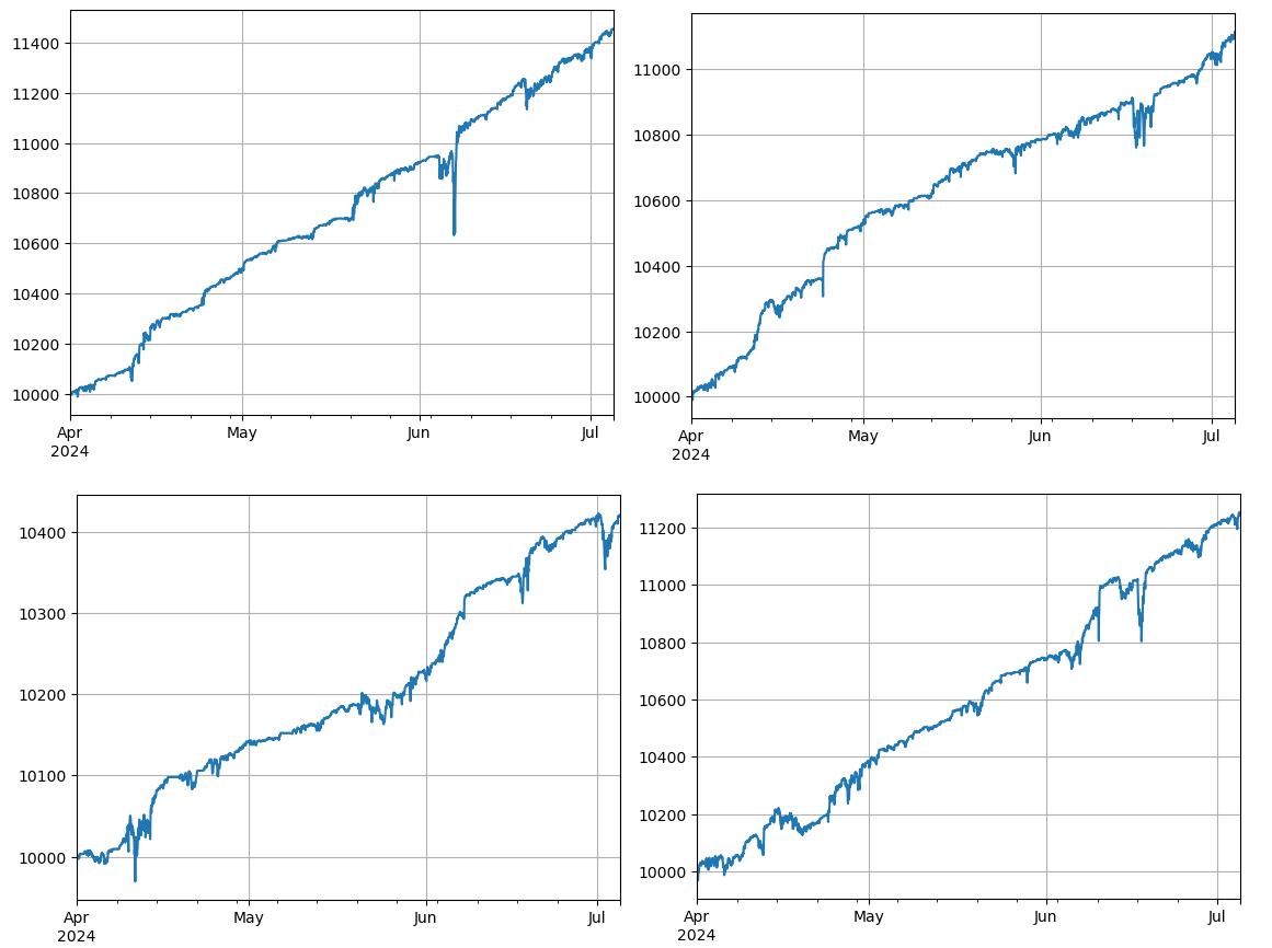
res['total'].plot(grid=True);

A total of 4 groups of currencies were retested, with the result being relatively ideal. The calculation of the current correlation is based on future data, so it is not very accurate. This article also divides the data into two parts, based on the correlation of the previous calculation, the retest of the latter.

Potential risks and ways to improve

Although pairing trading strategies can be profitable in theory, there are some risks in practical operation: correlations between currencies may change over time, causing the strategy to fail; price deviations may intensify under extreme market conditions, leading to larger losses; some currencies have low liquidity, which may make transactions difficult to execute or increase costs; and the handling fees generated by frequent trading may erode profits.

In order to reduce risk and improve the stability of the strategy, the following improvements can be considered: regularly recalculate the correlation between currency pairs, timely adjustment of trading pairs; set stop-loss and stop-loss points, controlling the maximum loss of a single trade; simultaneously trade multiple currency pairs, spreading the risk.

Conclusions

The digital currency pairing trading strategy is profitable by exploiting the correlation between the price of a currency and using leverage when the price deviates. The strategy has a high theoretical feasibility. A simple real-world strategy source code based on the strategy will then be released. If you have any further questions or need further discussion, please feel free to contact us.