Smooth Volatility Band Strategy

Overview

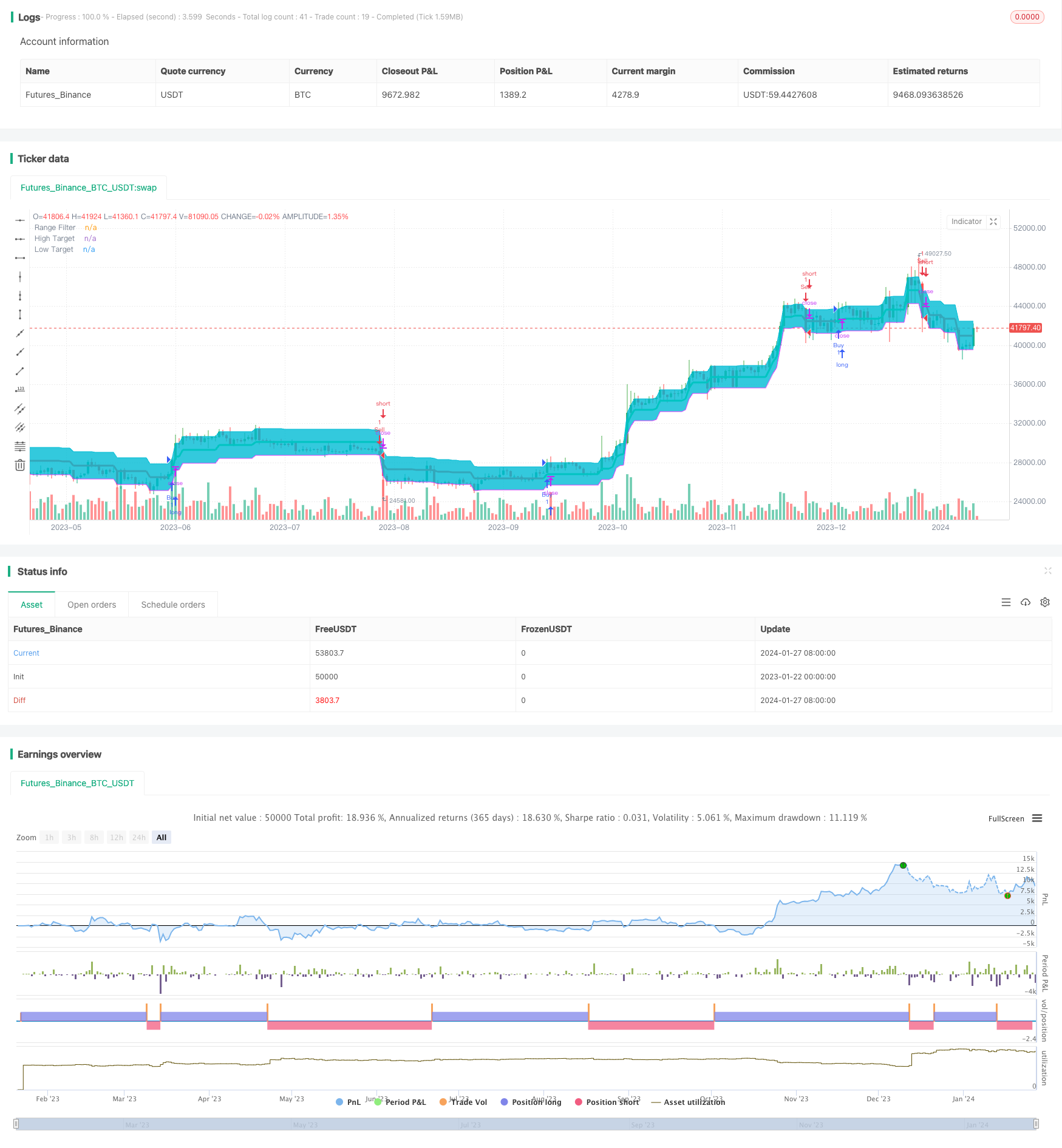
This strategy generates price bands based on the smoothed volatility of price, and produces trading signals when price breaks through the bands.

Strategy Logic

The strategy first calculates the average volatility range of price over a certain period, then smoothes the volatility range using an exponential moving average to generate smoothed volatility. The smoothed volatility multiplied by a coefficient gives the range of the bands. When price breaks above the upper band, a buy signal is generated. When price breaks below the lower band, a sell signal is generated.

Specifically, the smoothed volatility smrng is calculated by the smoothrng function. The upper band hband and lower band lband of the price bands are then calculated based on smrng. The long condition longCondition and short condition shortCondition are set up based on that. When longCondition is met, a buy signal is generated. When shortCondition is met, a sell signal is generated.

Advantage Analysis

The advantages of this strategy are:

1. Using price volatility to construct trading signals can effectively track market changes.

2. Smoothing volatility with exponential moving average can filter noise and generate more reliable trading signals.

3. The range of bands can be adjusted through the volatility coefficient, making the strategy more flexible.

4. Combined with breakout judgment, it can capture trading opportunities timely when trend reversal occurs.

Risk Analysis

There are also some risks in this strategy:

1. In abnormal market volatility, the smoothed volatility may fail to accurately reflect the actual volatility, leading to wrong signals. Parameters can be optimized to improve the model.

2. Improper band range setting may lead to overtrading or insufficient signals. Different parameters can be tested to find the optimal range.

3. There is time lag in breakout signals, which may cause premature entry or late entry. Other indicators can be introduced for confirmation.

Optimization Directions

The strategy can be optimized through:

1. Testing different price data cycles to find the most appropriate period for calculating volatility.

2. Trying different moving average algorithms like weighted moving average.

3. Introducing trading volume or other indicators to confirm breakout signals.

4. Setting stop loss or trailing stop to control losses per trade.

5. Optimizing the volatility coefficient mult to determine optimal band range.

Summary

The overall logic of this strategy is clear, using price volatility to construct bands and price breakouts to generate trading signals, which can effectively track market trend changes. But there is room for improvement via parameter optimization, signal confirmation etc to make strategy more robust.