Ornstein-Uhlenbeck simulation with Python

In this article, we will outline the Ornstein-Uhlenbeck process, describe its mathematical formulas, implement and simulate it using Python, and discuss some practical applications in quantitative finance and systemic trading. We will use a more advanced random process model, called the Ornstein-Uhlenbeck (OU) process, which can be used to model time sequences that exhibit even-valued regression behavior. This is particularly useful for interest rate modeling in derivative pricing and for algorithms for systemic trading when trading.

What is the Ornstein-Uhlenbeck process?

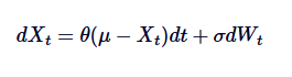
The Ornstein-Uhlenbeck process is a continuous-time random process used to model mean-valued regression behavior. This means that, unlike standard random walk or Brownian motion, which can drift indefinitely, the OU process tends to recover to a long-term mean over time. Mathematically, the OU process is a solution to a specific random differential equation (SDE) that controls such mean-valued regression behavior.

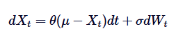
Here, Xt represents a random process at time t, where μ is the long mean,θ is the mean regression rate,δ is the volatility, and dWt is the Wiener process or standard Brownian motion.

Historical context and application

The Ornstein-Uhlenbeck process was originally proposed by Leonard Ornstein and George Eugene Uhlenbeck in 1930 to simulate the velocity of Brownian motion of particles in the presence of friction. Over time, its utility has extended far beyond physics and has been applied in a variety of fields, including biology, chemistry, economics, and finance.

In quantitative finance, the OU process is particularly useful for modeling phenomena that exhibit mean value regression behavior. Notable examples include interest rates, exchange rates, and volatility in financial markets. For example, the popular interest rate model, the Vasicek model, is derived directly from the OU process.

Importance of quantitative finance

The Ornstein-Uhlenbeck process is important in quantitative finance for the following reasons. Its average-value regression nature makes it a natural choice for modeling financial variables that do not exhibit random drift but instead fluctuate around stable long-term averages. This property is important for interest rate modeling, where the average-value regression reflects the central bank's influence on long-term stable interest rates.

In addition, the OU process is used in asset pricing models (including derivatives valuation) and risk management strategies. It can also be used as a building block for more complex models, such as the Cox-Ingersoll-Ross (CIR) model, which extends the OU process to model non-negative interest rates.

Main features and intuition

The main features of the Ornstein-Uhlenbeck process can be summarized as follows:

• The mean value of the regression is:The OU process tends to return to the long-term mean μ. This is in stark contrast to processes such as Brownian motion, which do not show this trend.
• The volatility:The parameter δ controls the level of randomness or volatility in the process. The higher the volatility, the greater the deviation from the mean before the process returns.
• The speed of return:The parameter θ determines the speed at which the process returns to the mean. The higher the value of θ, the faster the speed of the mean returns.
• Stability:The OU process is smooth, which means that its statistical characteristics do not change over time. This is crucial for modeling stable systems in the financial sector.

Intuitively, you can think of the Ornstein-Uhlenbeck process as modeling the behavior of elastic muscles stretching around the mean. Although the process may deviate from the mean due to random fluctuations, the elasticity of elasticity of the muscles (similar to the mean return) ensures that it eventually returns to the mean.

Comparison with other random processes

Because the OU process is closely related to the modeling of various financial phenomena, it is often compared to other random processes (such as Brownian motion and geometric Brownian motion (GBM)). Unlike Brownian motion (which has no uniform regression trend), the OU process has a distinct uniform regression behavior. This makes it more suitable for modeling scenarios in which variables fluctuate around a stable equilibrium.

Compared to GBM, which is typically used to model stock prices and contains drift and volatility items, the OU process does not show exponential growth, but rather fluctuations around its mean. The GBM is better suited to modeling quantities that grow over time, while the OU process is well suited to modeling variables that show mean regression characteristics.

Examples of quantitative finance

The Ornstein-Uhlenbec process has a wide range of applications in finance, especially in modeling scenarios where mean value regression is a key feature. We will discuss some of the most common use cases below.

Interest rate modeling

One of the most prominent applications of the OU process is modeling interest rates, especially within the framework of the Vasicek model. The Vasicek model assumes that interest rates follow the OU process, i.e. that interest rates tend to return to long-term averages over time. This feature is crucial for accurately modeling interest rate behavior, as interest rates often do not fluctuate indefinitely, but fluctuate near the average level as influenced by economic conditions.

Asset pricing

In asset pricing, especially fixed income securities, the OU process is often used to simulate the evolution of bond yields. The regressive nature of the OU process ensures that the yield does not deviate too far from its historical average, which is consistent with observed market behavior. This makes the OU process a valuable tool for pricing bonds and other rate-sensitive instruments.

Pairing trading strategies

Pairing trading is a market-neutral strategy that involves establishing offsetting positions in two related assets. In this case, the OU process is particularly useful because it can model the price difference between the two assets, where the price difference is usually a mean return. By modeling the price difference using the OU process, traders can identify the point of profit entry and exit when the price difference deviates from their average, predict the mean return, and thus generate a trading signal.

For example, if the spread between two futures expands beyond a certain threshold, traders may swap excellent futures for poor futures, expecting the spread to return to its historical average, thus making a profit when the reversal occurs.

The answer is Ornstein-Uhlenbeck SDE

The differential equation of the Ornstein-Uhlenbeck process is the basis for its solution. To solve this SDE, we use the integral factorization. Let's rewrite SDE:

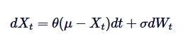
First, we multiply both sides by their factors. :

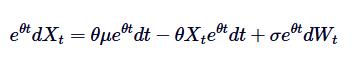
And notice, if we add both sides of this equation.So the left-hand side can be represented as the difference of the product:

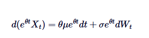
Let's take both sides from 0 to t, and we get:

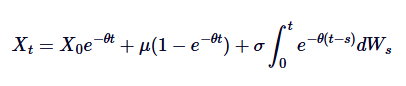
This is a general solution of the Ornstein-Uhlenbeck SDE.

The above deduced explicit solutions have several important implications.Indicates how the initial value decreases over time and how the process gradually forgets where it started.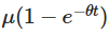The third term introduces randomness, in which the exponents involved in the Wiener process explain random fluctuations.

This solution emphasizes the balance between the regression behaviour of the mean of certainty and the random fraction driven by Brownian motion. Understanding this solution is crucial for effective simulation of OU processes, as described below.

Connections to other random processes

The Ornstein-Uhlenbeck process has several important links to other well-known random processes (including Brownian motion and the Vasicek model).

Relationship to the Brown Movement

The Ornstein-Uhlenbeck process can be thought of as an average regression version of the Brownian motion. The Brownian motion describes a trend with independent increment and no regression equation, while the OU process introduces an average regression by modifying the Brownian motion using a drift term, thus pulling the process back to the center value. Mathematically, if we set θ=0, the OU process will be simplified to a standard Brownian motion with oscillations:

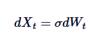
Thus, the Brownian motion is an exceptional case of the OU process, corresponding to the absence of a mean-valued regression.

Relationship to the Vasicek model

The Vasicek model is widely used in interest rate modeling, essentially as an application of the Ornstein-Uhlenbeck process in interest rate evolution. The Vasicek model assumes that interest rates follow the OU process, where SDE is defined as:

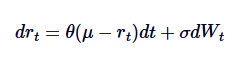
Among them, rt represents the short-term interest rate, the interpretation of the parameters θ, μ and δ is similar to the interpretation in the OU process. The Vasicek model is able to generate a mean-return interest rate path, which is one of its main advantages in financial modeling.

Understanding these relationships allows a broader understanding of how OU processes are used in different contexts, especially in the financial sector. We will explore the practical implications of these relationships when discussing application examples below.

Simulating the Ornstein-Uhlenbeck process with Python

In this section, we will explore how to use Python to simulate the Ornstein-Uhlenbeck (OU) process. This involves using Euler-Maruyama decomposition to decompose the random differential equation (SDE) that defines the OU process.

Diversification of the SDE

Let's review the SDE mathematical formula above and summarize each term:

In this case,

• Xt is the value of the process at time t.
• θ is the rate of return of the mean.
• μ is the long-term average of the process.
• δ is the frequency parameter.
• dWt represents the increment of the Wiener process (Standard Brownian motion).

In order to simulate this process on a computer, we need to do a discrete SDE of continuous time. A commonly used method is Euler-Maruyama discretion, which takes into account small discrete time steps.The discrete form of the Ornstein-Uhlenbeck process is given by:

In this case,is a random variable extracted from a standard normal distribution (i.e.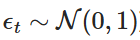This decoupling allows us to iteratively compute the value of Xt over time to simulate the behavior of the OU process.

Implementation of Python

Now let's implement a decentralized Ornstein-Uhlenbeck process in Python. In the following, we only use NumPy and the Matplotlib Python library.

First, we import NumPy and Matplotlib in the standard way. Then, we assign all the parameters to the OU model. Next, we pre-assign a NumPy array of length N to be added to it after calculating the OU path. Then we iterate through N-1 steps (step 1 is the initial condition X0 for the designation), simulate random increment dW, and then calculate the next iteration of the OU path using the above mathematical formula.

import numpy as np
import matplotlib.pyplot as plt

# Parameters for the OU process
theta = 0.7      # Speed of mean reversion
mu = 0.0         # Long-term mean
sigma = 0.3      # Volatility
X0 = 1.0         # Initial value
T = 10.0         # Total time
dt = 0.01        # Time step
N = int(T / dt)  # Number of time steps

# Pre-allocate array for efficiency
X = np.zeros(N)
X[0] = X0

# Generate the OU process
for t in range(1, N):
    dW = np.sqrt(dt) * np.random.normal(0, 1)
    X[t] = X[t-1] + theta * (mu - X[t-1]) * dt + sigma * dW

# Plot the result
plt.plot(np.linspace(0, T, N), X)
plt.title("Ornstein-Uhlenbeck Process Simulation")
plt.xlabel("Time")
plt.ylabel("X(t)")
plt.show()

The results of the drawings are as follows:

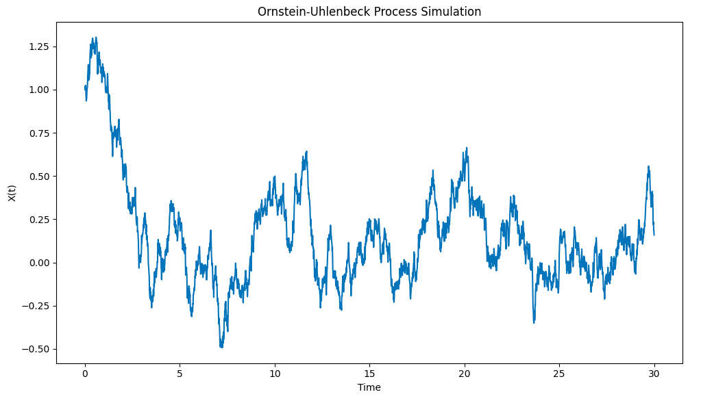
Ornstein-Uhlenbeck process simulation drawn with Python

Notice how the process quickly pulls a particle X0=1 from the initial condition to the mean μ=0, and then shows a tendency to return to that mean when it deviates from that mean.

Summary and follow-up

In this article, we outline the Ornstein-Uhlenbeck process, describe its mathematical formulas, and provide a basic implementation of Python to simulate discrete versions of continuous-time SDEs. In subsequent articles, we will explore more complex SDEs built based on OU processes and how they can be used in system trading and derivative pricing applications.

Full code

# OU process simulation

import numpy as np
import matplotlib.pyplot as plt

# Parameters for the OU process
theta = 0.7      # Speed of mean reversion
mu = 0.0         # Long-term mean
sigma = 0.3      # Volatility
X0 = 1.0         # Initial value
T = 30.0         # Total time
dt = 0.01        # Time step
N = int(T / dt)  # Number of time steps

# Pre-allocate array for efficiency
X = np.zeros(N)
X[0] = X0

# Generate the OU process
for t in range(1, N):
    dW = np.sqrt(dt) * np.random.normal(0, 1)
    X[t] = X[t-1] + theta * (mu - X[t-1]) * dt + sigma * dW

# Plot the result
plt.plot(np.linspace(0, T, N), X)
plt.title("Ornstein-Uhlenbeck Process Simulation")
plt.xlabel("Time")
plt.ylabel("X(t)")
plt.show()

The original link:https://www.quantstart.com/articles/ornstein-uhlenbeck-simulation-with-python/