Recursive Momentum Trading Strategy
Author: ChaoZhang, Date: 2024-01-31 16:56:31Tags:

Overview
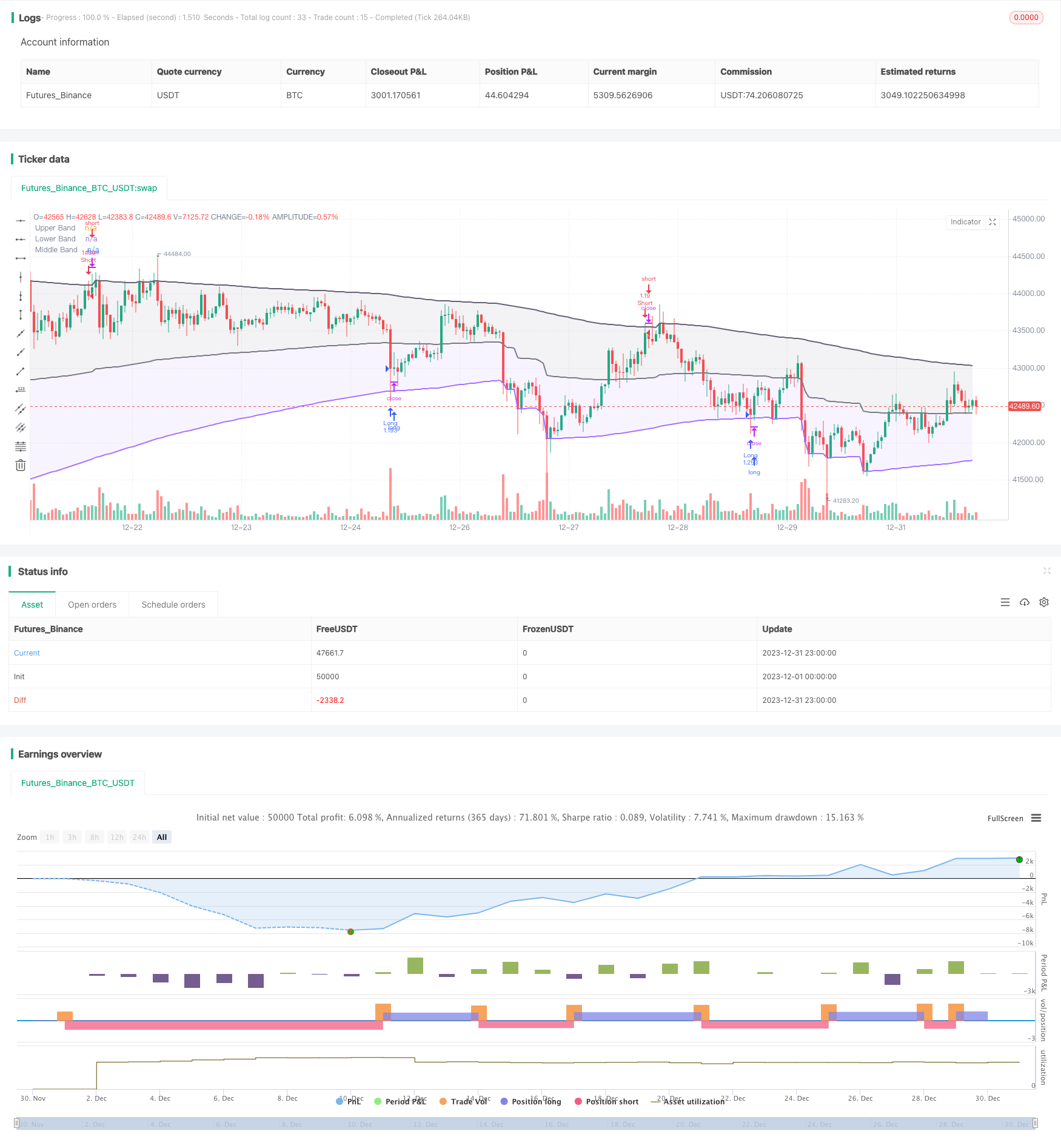
This strategy is a trend-following and breakout strategy based on the Recursive Bands indicator developed by alexgrover. It uses the Recursive Bands indicator to determine price trends and key support/resistance levels, combined with momentum conditions to filter out false breakouts, achieving low-frequency but high-quality entry signals.
Strategy Logic
Recursive Bands Indicator Calculation
The Recursive Bands indicator consists of an upper band, lower band and middle line. The indicator is calculated as:
Upper Band = Max(Previous bar’s upper band, Close price + n*Volatility) Lower Band = Min(Previous bar’s lower band, Close price - n*Volatility) Middle Line = (Upper Band + Lower Band)/2
Here n is a scaling coefficient, and volatility can be chosen from ATR, standard deviation, average true range or a special RFV method. The length parameter controls the sensitivity, larger values make the indicator trigger less frequently.
Trading Rules
The strategy first checks if the lower band and upper band are trending in the same direction to avoid false breakouts.
When price breaks below the lower band, go long. When price breaks above the upper band, go short.
In addition, stop loss logic is implemented.
Advantage Analysis
The advantages of this strategy are:
- Efficient indicator calculation using recursive framework, avoiding repeated computation
- Flexible parameter tuning to adapt to different market regimes
- Combining trend and breakout, avoiding false breakouts
- Momentum condition filters ensure signal quality
Risk Analysis
There are also some risks with this strategy:
- Improper parameter settings may lead to overtrading or poor signal quality
- May face large losses when major trend changes
- Insufficient slippage control in extreme moves may amplify losses
These risks can be managed by parameter optimization, implementing stop loss, increasing slippage threshold etc.
Optimization Directions
Some directions to optimize the strategy further:
- Incorporate indicators across multiple timeframes for robustness
- Add machine learning module for adaptive parameter optimization
- Conduct quantitative correlation analysis to find optimal parameter combinations
- Use deep learning to forecast price paths and improve signal accuracy
Conclusion
In summary, this is a very practical and efficient trend-following strategy. It combines the recursive framework for computational efficiency, uses trend support/resistance to determine major trends, adds momentum conditions to filter false breakouts and ensure signal quality. With proper parameter tuning and risk control, it can achieve good results. Worthy of further research and optimization to adapt to more complex market regimes.
/*backtest
start: 2023-12-01 00:00:00
end: 2023-12-31 23:59:59
period: 1h
basePeriod: 15m
exchanges: [{"eid":"Futures_Binance","currency":"BTC_USDT"}]
*/

// @version=5
// Original indicator by alexgrover
strategy('Extended Recursive Bands Strategy', overlay=true, commission_type=strategy.commission.percent,commission_value=0.06,default_qty_type =strategy.percent_of_equity,default_qty_value = 100,initial_capital =1000)
length = input.int(260, step=10, title='Length')
src = input(close, title='Source')
method = input.string('Classic', options=['Classic', 'Atr', 'Stdev', 'Ahlr', 'Rfv'], title='Method')
bandDirectionCheck = input.bool(true, title='Bands Hold Direction')
lookback = input(3)
//----
atr = ta.atr(length)
stdev = ta.stdev(src, length)
ahlr = ta.sma(high - low, length)
rfv = 0.
rfv := ta.rising(src, length) or ta.falling(src, length) ? math.abs(ta.change(src)) : rfv[1]
//-----
f(a, b, c) =>
    method == a ? b : c
v(x) =>
    f('Atr', atr, f('Stdev', stdev, f('Ahlr', ahlr, f('Rfv', rfv, x))))
//----
sc = 2 / (length + 1)
a = 0.
a := math.max(nz(a[1], src), src) - sc * v(math.abs(src - nz(a[1], src)))
b = 0.
b := math.min(nz(b[1], src), src) + sc * v(math.abs(src - nz(b[1], src)))
c = (a+b)/2

// Colors
beColor = #675F76
buColor = #a472ff

// Plots
pA = plot(a, color=color.new(beColor, 0), linewidth=2, title='Upper Band')
pB = plot(b, color=color.new(buColor, 0), linewidth=2, title='Lower Band')
pC = plot(c, color=color.rgb(120,123,134,0), linewidth=2, title='Middle Band')
fill(pC, pA, color=color.new(beColor,90))
fill(pC, pB, color=color.new(buColor,90))

// Band keeping direction
// By Adulari
longc = 0
shortc = 0
for i = 0 to lookback-1
    if b[i] > b[i+1]
        longc:=longc+1
    if a[i] < a[i+1]
        shortc:=shortc+1
bhdLong = if bandDirectionCheck
    longc==lookback
else
    true
bhdShort = if bandDirectionCheck
    shortc==lookback
else
    true

// Strategy
if b>=low and bhdLong
    strategy.entry(id='Long',direction=strategy.long)
if high>=a and bhdShort
    strategy.entry(id='Short',direction=strategy.short)

// TP at middle line
//if low<=c and strategy.position_size<0 and strategy.position_avg_price>close
    //strategy.exit(id="Short",limit=close)
//if high>=c and strategy.position_size>0 and strategy.position_avg_price<close
    //strategy.exit(id="Long",limit=close)
- Breakback Storm Strategy in Hidden Opportunities
- Cross-Timeframe Momentum Tracking Strategy
- Moving Average Trend Following Strategy
- Pivot SuperTrend Strategy Across Multiple Timeframes
- Quantitative Candlestick Pattern and Trend Following Strategy
- Supertrend Combined with RSI Quantitative Trading Strategy
- Cape Town 15-min Candle Breakout Strategy
- Dual ATR Trailing Stop Strategy
- Qullamaggie Breakout Tracking Strategy
- Extreme version of Noro's Trend Moving Averages Strategy
- Donchian Trend Following Strategy
- SuperTrend RSI EMA Crossover Strategy
- Bilateral Three-Point Moving Average Quantitative Trading Strategy
- Trading Strategy Based on RSI and MACD Indicators
- CCI and EMA Based Scalping Strategy
- Improved Wave Trend Tracking Strategy
- Ichimoku Entries Strategy
- Trend Following Strategy Based on Moving Average Crossover
- RSI Trend Following Strategy with Trailing Stop Loss
- Consolidation Breakout Strategy