概述
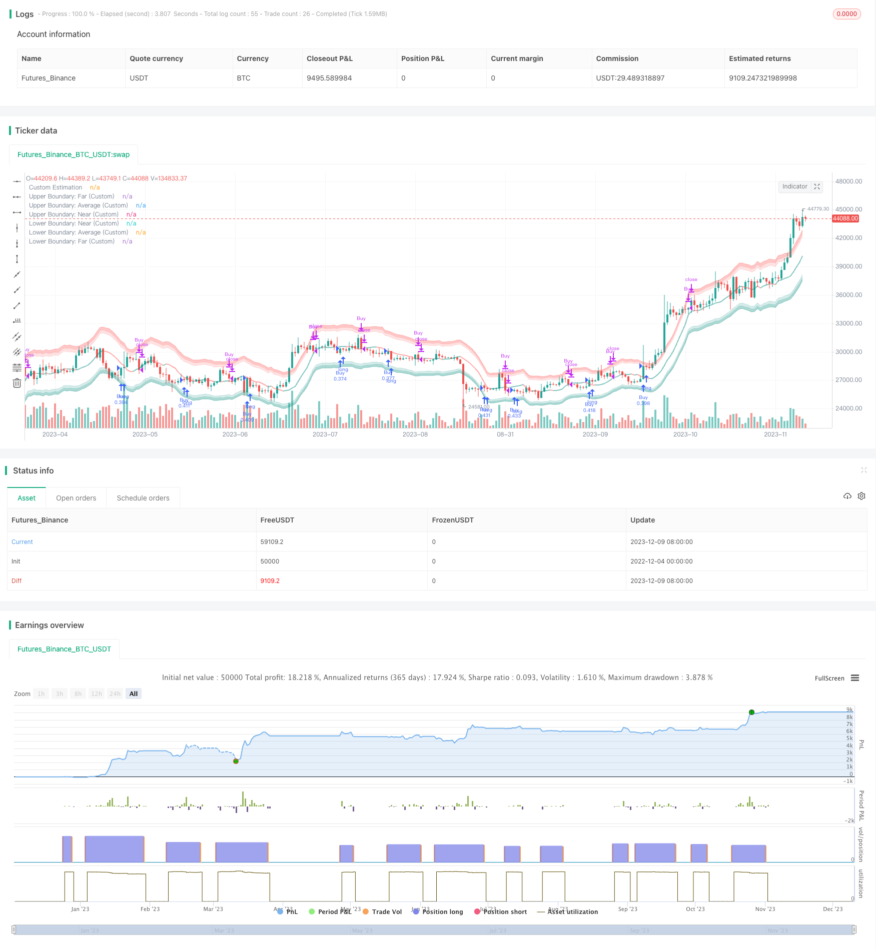
该策略基于Nadaraya-Watson核回归方法构建了一个动态波动率包围带,通过跟踪价格与包围带的交叉情况,实现低买高卖的交易信号。策略具有数学分析基础,能够自适应市场变化。
策略原理
策略的核心是计算价格的动态包围带。首先,根据自定义的看回期,构建价格(收盘价、最高价、最低价)的Nadaraya-Watson核回归曲线,得到平滑化的价格估计。然后基于自定义的ATR长度计算ATR指标,结合近端因子和远端因子,得到上下包围带的范围。当价格从下包围带下方突破进入包围带,产生买入信号;当价格从上包围带上方突破离开包围带,产生卖出信号。该策略通过跟踪价格与波动率相关的统计属性,动态调整交易决策。
策略优势
- 基于数学模型,参数可控,不容易产生过度优化
- 自适应市场变化,利用价格与波动率的动态关系捕捉交易机会
- 采用对数坐标,能够很好处理不同时间周期和波动幅度的品种
- 可自定义参数调整策略的灵敏度
策略风险
- 数学模型理论化,实盘表现可能不如预期
- 关键参数选取需要经验,不当设置可能影响收益
- 存在一定的滞后,可能错过部分交易机会
- 大幅震荡市场中容易出现错误信号
主要通过优化参数,做好回测,了解影响因素,谨慎实盘来规避和减少这些风险。
策略优化方向
- 进一步优化参数,找出最佳参数组合
- 利用机器学习方法自动优选参数
- 增加过滤条件,在特定市场环境下激活策略
- 结合其他指标过滤误导信号
- 尝试不同的数学模型算法
总结
该策略整合统计分析与技术指标分析,通过动态跟踪价格与波动率,实现低买高卖的交易信号。可根据市场和自身情况调整参数。整体来说,策略理论基础坚实,实际表现还有待进一步验证。需要谨慎看待,审慎实盘。
策略源码
/*backtest
start: 2022-12-04 00:00:00
end: 2023-12-10 00:00:00
period: 1d
basePeriod: 1h
exchanges: [{"eid":"Futures_Binance","currency":"BTC_USDT"}]
*/

// © Julien_Eche
//@version=5

strategy("Nadaraya-Watson Envelope Strategy", overlay=true, pyramiding=1, default_qty_type=strategy.percent_of_equity, default_qty_value=20)

// Helper Functions
getEnvelopeBounds(_atr, _nearFactor, _farFactor, _envelope) =>
    _upperFar = _envelope + _farFactor*_atr
    _upperNear = _envelope + _nearFactor*_atr
    _lowerNear = _envelope - _nearFactor*_atr
    _lowerFar = _envelope - _farFactor*_atr
    _upperAvg = (_upperFar + _upperNear) / 2
    _lowerAvg = (_lowerFar + _lowerNear) / 2
    [_upperNear, _upperFar, _upperAvg, _lowerNear, _lowerFar, _lowerAvg]

customATR(length, _high, _low, _close) =>
    trueRange = na(_high[1])? math.log(_high)-math.log(_low) : math.max(math.max(math.log(_high) - math.log(_low), math.abs(math.log(_high) - math.log(_close[1]))), math.abs(math.log(_low) - math.log(_close[1])))
    ta.rma(trueRange, length)

customKernel(x, h, alpha, x_0) =>
    sumWeights = 0.0
    sumXWeights = 0.0
    for i = 0 to h
        weight = math.pow(1 + (math.pow((x_0 - i), 2) / (2 * alpha * h * h)), -alpha)
        sumWeights := sumWeights + weight
        sumXWeights := sumXWeights + weight * x[i]
    sumXWeights / sumWeights

// Custom Settings
customLookbackWindow = input.int(8, 'Lookback Window (Custom)', group='Custom Settings')
customRelativeWeighting = input.float(8., 'Relative Weighting (Custom)', step=0.25, group='Custom Settings')
customStartRegressionBar = input.int(25, "Start Regression at Bar (Custom)", group='Custom Settings')

// Envelope Calculations
customEnvelopeClose = math.exp(customKernel(math.log(close), customLookbackWindow, customRelativeWeighting, customStartRegressionBar))
customEnvelopeHigh = math.exp(customKernel(math.log(high), customLookbackWindow, customRelativeWeighting, customStartRegressionBar))
customEnvelopeLow = math.exp(customKernel(math.log(low), customLookbackWindow, customRelativeWeighting, customStartRegressionBar))
customEnvelope = customEnvelopeClose
customATRLength = input.int(60, 'ATR Length (Custom)', minval=1, group='Custom Settings')
customATR = customATR(customATRLength, customEnvelopeHigh, customEnvelopeLow, customEnvelopeClose)
customNearATRFactor = input.float(1.5, 'Near ATR Factor (Custom)', minval=0.5, step=0.25, group='Custom Settings')
customFarATRFactor = input.float(2.0, 'Far ATR Factor (Custom)', minval=1.0, step=0.25, group='Custom Settings')
[customUpperNear, customUpperFar, customUpperAvg, customLowerNear, customLowerFar, customLowerAvg] = getEnvelopeBounds(customATR, customNearATRFactor, customFarATRFactor, math.log(customEnvelopeClose))

// Colors
customUpperBoundaryColorFar = color.new(color.red, 60)
customUpperBoundaryColorNear = color.new(color.red, 80)
customBullishEstimatorColor = color.new(color.teal, 50)
customBearishEstimatorColor = color.new(color.red, 50)
customLowerBoundaryColorNear = color.new(color.teal, 80)
customLowerBoundaryColorFar = color.new(color.teal, 60)

// Plots
customUpperBoundaryFar = plot(math.exp(customUpperFar), color=customUpperBoundaryColorFar, title='Upper Boundary: Far (Custom)')
customUpperBoundaryAvg = plot(math.exp(customUpperAvg), color=customUpperBoundaryColorNear, title='Upper Boundary: Average (Custom)')
customUpperBoundaryNear = plot(math.exp(customUpperNear), color=customUpperBoundaryColorNear, title='Upper Boundary: Near (Custom)')
customEstimationPlot = plot(customEnvelopeClose, color=customEnvelope > customEnvelope[1] ? customBullishEstimatorColor : customBearishEstimatorColor, linewidth=2, title='Custom Estimation')
customLowerBoundaryNear = plot(math.exp(customLowerNear), color=customLowerBoundaryColorNear, title='Lower Boundary: Near (Custom)')
customLowerBoundaryAvg = plot(math.exp(customLowerAvg), color=customLowerBoundaryColorNear, title='Lower Boundary: Average (Custom)')
customLowerBoundaryFar = plot(math.exp(customLowerFar), color=customLowerBoundaryColorFar, title='Lower Boundary: Far (Custom)')

// Fills
fill(customUpperBoundaryFar, customUpperBoundaryAvg, color=customUpperBoundaryColorFar, title='Upper Boundary: Farmost Region (Custom)')
fill(customUpperBoundaryNear, customUpperBoundaryAvg, color=customUpperBoundaryColorNear, title='Upper Boundary: Nearmost Region (Custom)')
fill(customLowerBoundaryNear, customLowerBoundaryAvg, color=customLowerBoundaryColorNear, title='Lower Boundary: Nearmost Region (Custom)')
fill(customLowerBoundaryFar, customLowerBoundaryAvg, color=customLowerBoundaryColorFar, title='Lower Boundary: Farmost Region (Custom)')


longCondition = ta.crossover(close, customEnvelopeLow)
if (longCondition)
    strategy.entry("Buy", strategy.long)

exitLongCondition = ta.crossover(customEnvelopeHigh, close)
if (exitLongCondition)
    strategy.close("Buy")